In graphics and machine learning conversations, a tensor is a block of numbers with a shape: a list of sizes, one per axis, that tells you how many indices you need to find a single value and how far each index can go. A matrix is a tensor with two axes, and if you have ever worked with a texture you have already handled a tensor with three, height by width by channels, so the word is less new than it sounds, and the reason it keeps coming up is that renderers now run small neural networks inside the frame, for denoising, upscaling and caching lighting, and those networks are written entirely in terms of tensors.
This primer is for a technical artist who is comfortable with matrices and textures and has never needed to go past three axes. It builds the idea up from the texture you already know, shows the shapes we actually use in Breda's neural network crate, breda-nn, works through one layer of a real network with its numbers, and says where the everyday meaning of the word departs from the mathematical one.
Last updated 2026-10-02.
Rank is the number of indices
A single number needs no index to find it, a list of 48 numbers needs one, a 64 by 48 grid needs two, and an RGBA image needs three: which row, which column, which channel. That count of indices is the tensor's rank, and its shape lists how long each axis is, so a 1920 by 1080 RGBA image has rank 3 and shape [1080, 1920, 4], and nothing about it changes when someone starts calling it a tensor instead of a texture.
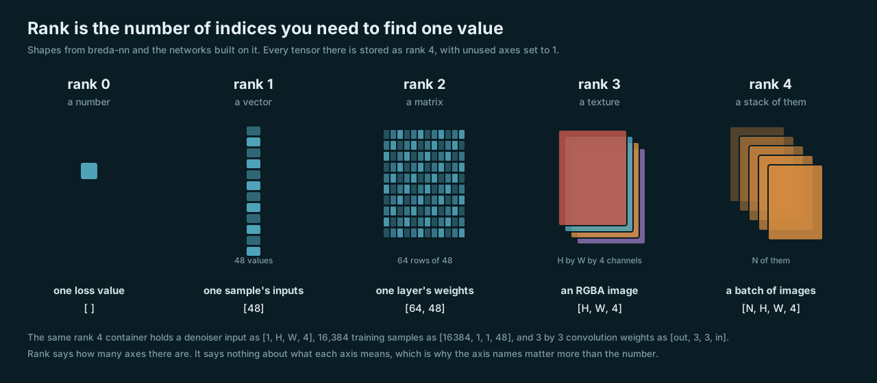
Ranks 0 to 4, with shapes from breda-nn and the networks built on it.
Two of the words used so far mean something else in neighbouring fields: in linear algebra the rank of a matrix is the number of independent rows it has rather than its number of axes, which is why some libraries say "order" or "number of dimensions" for what this post calls rank, and in physics and mathematics a tensor is a stricter object than a block of numbers. The inertia tensor in a physics engine, for example, is a 3 by 3 grid that must change in one specific way when the body rotates, and that rule is part of what makes it a tensor, while machine learning code carries no such rule: its tensors are arrays with a shape and nothing more, and that is the sense every rendering conversation about neural networks uses.
The fourth axis is usually "how many"
Going from three axes to four sounds like a leap into something you cannot picture, and it almost never is, because the fourth axis is nearly always a count: how many images, how many samples, how many filters. A stack of 16 RGBA images of the same size is a rank 4 tensor with shape [16, H, W, 4], which is exactly what a texture array is, and the letters people use for those axes, N for the count, H and W for height and width and C for channels, are the whole vocabulary you need to read most of the shapes in a network.
breda-nn makes that literal: every tensor it creates has exactly four axes, n, h, w and c, and anything that needs fewer simply sets the unused ones to 1. That is a convenience in the code, and it also shows that the same four slots can hold three quite different things:
| What it is | Shape | What the axes mean |
|---|---|---|
| Input to our denoiser | [1, H, W, 4] | one image, padded to a multiple of 16 pixels each way, RGB padded to four channels |
| One training batch for the radiance cache | [16384, 1, 1, 48] | 16,384 samples, no image at all, 48 numbers describing each one |
| Weights of a 3 by 3 convolution | [out, 3, 3, in] | one 3 by 3 filter for every pair of output and input channel |
The first is a texture in all but name, and the denoiser behind it is a reimplementation of Open Image Denoise that we wrote about in an earlier post, the second has height and width of 1, so despite its four axes it is really a list of 16,384 rows of 48 numbers, a matrix, and the third uses the "how many" axis to count output channels rather than images. Rank tells you how many axes there are and nothing about what they mean, so when you read a shape the useful question is what each axis is counting, not how many of them there are.
How four axes sit in one-dimensional memory
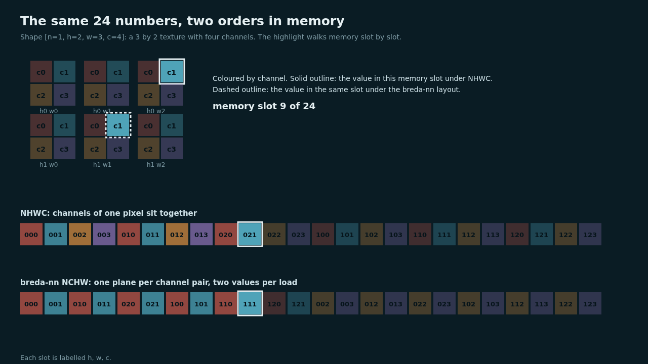
A GPU buffer is a flat run of bytes, so a tensor needs a rule for which value goes where, and there are two common answers that match something you already know from textures. NHWC keeps all the channels of one pixel together, the way an interleaved RGBA texture stores R, G, B and A side by side, and NCHW stores a whole plane for each channel, one image of reds and then one of greens, the way a planar format does. For NHWC, the position of the value at in a tensor of shape is
and NCHW is the same formula with the axes taken in a different order. Neither layout is more correct, they are faster for different operations, and breda-nn supports both, with a comment in its source noting that TensorFlow tends to use NHWC, PyTorch uses NCHW, and that we mostly start from PyTorch.
The layout our shaders use for NCHW has one more twist: our tensors store 16-bit floats, and the shaders read and write them two at a time, so instead of a plane per channel there is a plane per pair of channels with the two values of each pair side by side, which in the shader's own words is shape [n, c/2, h, w, 2]: still NCHW in spirit, but no longer the textbook version, and anyone moving data between our tensors and another tool has to know it.
A worked example: one layer of the radiance cache
Following one layer of a real network shows why tensors and matrices end up being the same conversation: Breda's neural radiance cache, an implementation of the technique from Müller and colleagues' 2021 paper, trains a small network while the renderer runs, to predict the light leaving points in the scene, and by default it does so in batches of 16,384 samples. Each sample is described by 48 numbers: 32 from a learned encoding of its position and 16 from the surface it sits on, such as its normal, the direction the light leaves in and its roughness.
So the input to the network is a tensor of shape [16384, 1, 1, 48], which, with its two unit axes dropped, is a matrix with 16,384 rows and 48 columns. The first layer's weights are stored as a [1, 1, 64, 48] tensor, a matrix with 64 rows and 48 columns, and the layer is a single matrix multiplication followed by an activation that clamps negative values to zero:
Every one of the 16,384 output rows is 64 dot products of length 48, which is multiply-adds for this one layer, and the network has six such layers: 48 to 64, four of 64 to 64, and 64 to 8 at the end.
The other numbers are smaller than people expect: the input batch at two bytes per value is bytes, 1.5 MiB, and the whole network's weights are
values, 39,936 bytes, which is less than a single 128 by 128 RGBA8 texture at 65,536 bytes. Training keeps further arrays of that size alongside, for gradients and the optimizer's state, and it is still small.
That is the case in miniature for why graphics programmers now talk about tensors: the work is a large number of small matrix multiplications over batches, which is a different shape of work from shading pixels, and the data is small enough to live close to the arithmetic.
Why the word keeps coming up
Two things have pulled the word into graphics. The first is the networks themselves: denoisers, upscalers and radiance caches all run inside the frame now, and every one of them is described by the shapes of the tensors flowing through it, so a technical conversation about any of them is partly a conversation about shapes and layouts.
The second is the hardware: recent GPUs include units built to multiply small matrices quickly, which some vendors market under the word tensor, and shading languages are gaining ways to reach them, such as the cooperative matrix extensions in Vulkan, which let a group of shader threads multiply a tile of one matrix by a tile of another as a single operation, and cooperative vectors, which do the same for a matrix times one vector per thread. The multi-layer network in breda-nn that the radiance cache runs on uses cooperative vectors by default and can use cooperative matrices instead, where the device supports them, which is exactly the worked example above handed to hardware designed for it.
None of this changes what a tensor is. When someone in a review says a tensor is "[16384, 1, 1, 48] in NHWC", they mean a list of 16,384 rows of 48 half-precision numbers with each row's values stored next to each other, and you now have everything you need to picture it, work out how big it is, and ask what each axis is counting.
What to read next
If you want to see tensors doing something visible, our posts on denoising ray traced images with Open Image Denoise and on neural radiance fields both show networks at work in a renderer, and the radiance cache paper linked above describes the network used in the worked example. For the layout question in more depth, the PyTorch tutorial on channels-last memory format explains the NCHW and NHWC trade from the machine learning side, with the same letters this post uses.