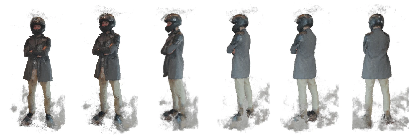
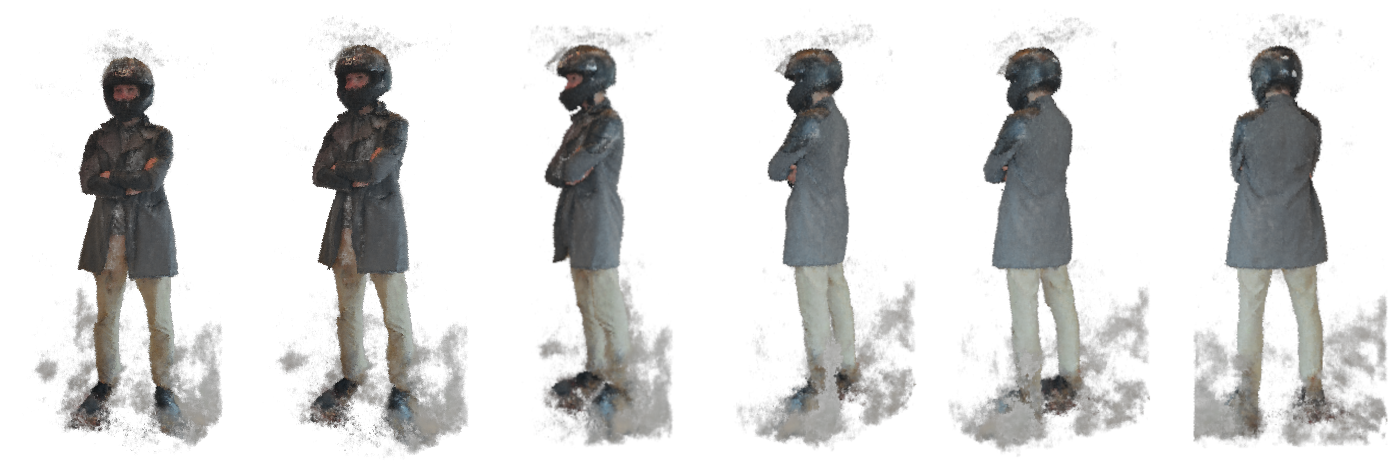
Angel Angelov visualized as a NeRF (Breda Framework)
Hi there, I’m Jason de Wolff. Currently, I am in my 2nd year at Breda University of Applied Sciences, I was offered to do an internship here at Traverse Researchduring the summer break. During these 8 weeks, my objective would be to recreate the rendering/inference of a NeRF inside the Breda framework. Obviously, I said yes.
This blog post goes over the basics of rendering a Neural Radiance Field (NeRF) inside the Breda rendering framework. It will also give an inside into the life of a traverse intern.
NeRF was first introduced here. Later NVidia published their Instant-NGP paper which significantly sped up the training process, NGP standing for neural graphics primitive. Our implementation is primarily based on the Instant-NGP paper.
Multi-resolution hash encoding
The main contributor to speeding up the training process is the multi-resolution hash encoding, which allows the neural network to learn details relatively well and quickly. The encoding consists of a sparse voxel representation, where each corner of the voxel grid is stored in a flat one-dimensional buffer. The encoding receives as input a 3D position which is used to sample and interpolate 8 vertices from the sparse 3D grid. This is done for *L *amount of layers, in our case 16. Each layer holds *N *parameters, in our case between 2¹⁴ and 2²⁴, depending on the size of the scene. Each layer has an increasing voxel size, determined by the *per_level_scale *parameter, in our case set to 1.5. The resolution of layer 0 is defined by base_resolution, set to 16.
The indexing into these parameters is done linearly when the resolution of the current layer doesn’t exceed the number of parameters it holds. Otherwise, a spatial hash function is used. Hash collisions are not treated as the neural network is responsible for countering these artifacts. Concatenating the outputs of the positional encoding reduces the artifacts further.
Every corner holds multiple values referred to as features, we use n_features = 2. These features are the actual learnable parameters. The interpolated corner values of every layer and its features are concatenated together and form the input of a dense Multi-Layer Perceptron (MLP).
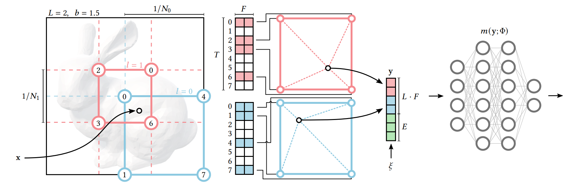
Multi-resolution hash encoding, from instantNGP
Code sample — see the original on Medium, linked at the end of this post.
Model setup
The NeRF from Instant-NGP consists out of 2 MLPs, a density, and a RGB MLP. The density MLP takes the encoded position as input and outputs 16 values, the first of which represents log-space density. The input of our RGB MLP takes the 16 output values from the density MLP and concatenates it with the spherically encoded ray direction (NeRFs are rendered using ray marching). This results in 32 input values for the RGB MLP. In our setup, we use 1 hidden layer of 64 neurons for the density network and 2 hidden layers of 64 neurons for the RGB network. The RGB network outputs an RGB color which uses a sigmoid activation function.
Rendering
A NeRF can be encapsulated by a bounding box. We march rays through this box with an exponentially increasing step size. At every step, we use an occupancy grid to get a rough idea if we need to take a sample there or not. If the occupancy grid hints that there’s something at this position, we query our entire model with the 3D position as input. The total query looks the following: (positional encoding -> density MLP + dir encoding) -> RGB MLP.
The occupancy grid helps speed up performance by a lot, as each query is very expensive. All samples along a ray are blended together to form the final output color for the corresponding pixel.

Expected color for a ray, from NeRF
Because the rendering is done with classical rays, effects such as depth of field or motion blur can be applied if desired.
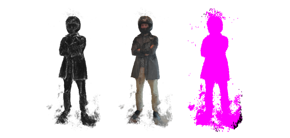
From left to right: density network, density + rgb network, occupancy grid (Breda Framework)
Breda framework
All of this is implemented inside the Breda framework. This framework uses a bindless approach to improve usability. It can be run either on our Vulkan or DX12 backend. To give an example of how easy it is to get a compute shader running, the following code executes a shader that plots all payloads from a buffer onto the render target texture.
Code sample — see the original on Medium, linked at the end of this post.
All compute and render passes are compiled in the render graph, which optimally reorders all passes for execution. After the render graph has been compiled it can be executed. And all of this, without the user needing to know any specific knowledge about the rendering API being used.
Conclusion
There’s a lot left to be done. We still want to implement training from 360 images and speed up rendering performance. By this time recent papers have also shown the potential for relighting NeRFs in real-time. For now, this serves as a solid foundation to work from.
As an intern, I had a lot of fun working at Traverse. The company culture is very nice and the codebase is a joy to work with. If you get the chance to work with these smart people, you should ;)