In this blog post, I’ll write about how I recreated the OIDN U-Net DNN using Rust and HLSL compute shaders, and about my time as an Intern at Traverse Research.
For some background, I’m Matt, a 2nd year Games programming student at the Breda University of Applied Sciences (BUAS). I’ve been programming for a couple of years, but this was the first time I’ve properly dipped my toes into machine learning, compute shaders, and working with a professional codebase.
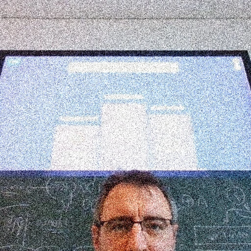
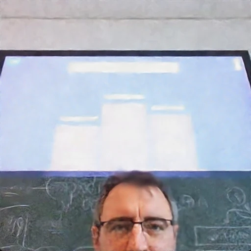
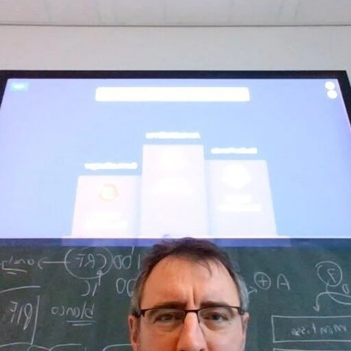
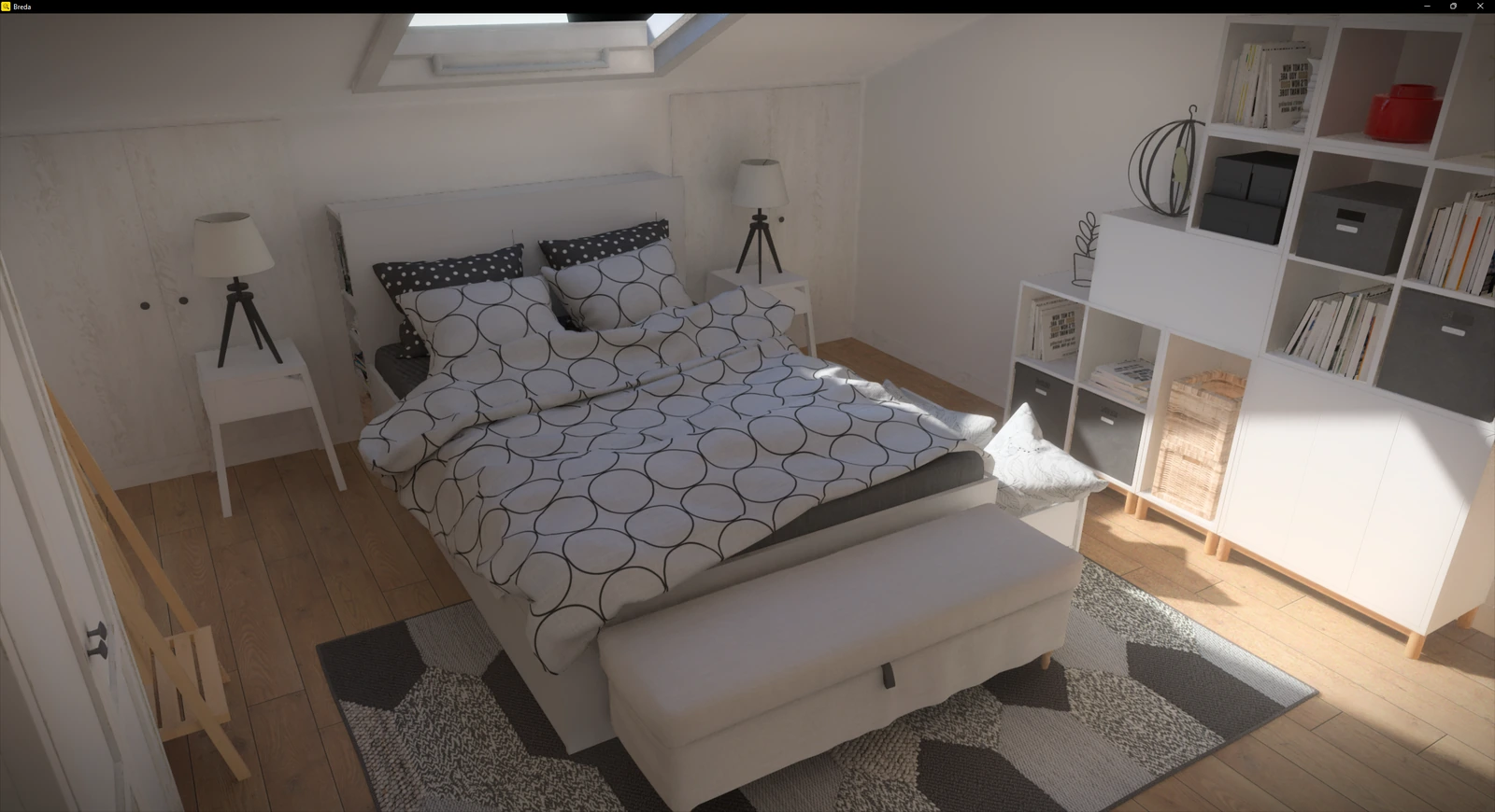
From left to right: noisy, denoised, and ground truth. (Using only a color image as input, kindly provided by our lecturer at BUAS Jacco Bikker)
What is OIDN
For brevity and clarity, I’ll quote Intel’s description of OIDN, which is “an open-source library of high-performance, high-quality denoising filters for images rendered with ray tracing”. The specific part I’ll be writing about is what the network is, the parts that are required for it to work, and how I went about optimizing my implementation.
The Network
Simplified down, the OIDN U-Net is just a series of weighted convolutions with extra steps, almost exactly like how you would implement a basic Gaussian blur. It’s called a U-Net because we downsample as we get further along (moving down), and then start upsampling halfway through (moving up), incorporating previous layers to maintain detail, which ends up making a U-shaped network if viewed as a diagram, otherwise it is just a regular neural network.
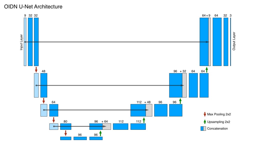
Diagram of the OIDN U-Net. Source: https://maxliani.wordpress.com/2023/04/07/dnnd-3-the-u-net-architecture/
In total, the OIDN U-Net has a whopping 43 operations, but of those, there are only 4 different types, convolution, max pooling, upsampling, and ReLU activation.
I’ll now go over each of the unique operations, in order of complexity.
ReLU
ReLU or “Rectified Linear Unit” is way simpler than the name makes it out to be, a ReLU activation simply returns the input value if it’s positive, otherwise returns 0 or the common max(0, input). That’s it.
Max Pooling and Upsampling
In our case, pooling is synonymous with downsampling to half resolution, so we take a 2x2 area of our image (a window if you will), select the highest value in the window (Max), and output that as our max pooled value. For upsampling we do something similarly simple, we just take each of our input values, and create a 2x2 area of the same value, doubling our resolution.
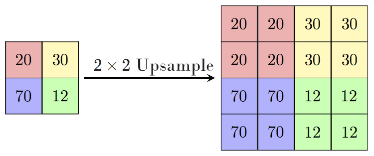
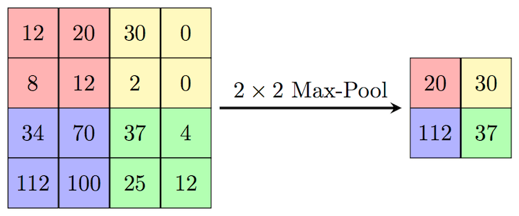
Source: https://computersciencewiki.org/images/8/8a/MaxpoolSample2.png?20180226194350
Convolution
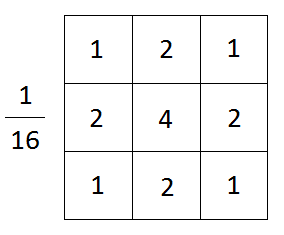
Convolutions in the context of images work slightly differently than they do in neural networks. Traditionally, you have a window with weights, that you slide over the image and multiply all the pixels in the area the window covers by their appropriate weights, and then sometimes add a value (called bias). With image filtering most of the time you apply the same weights to all channels of the image, and you usually only have 3 channels (RGB).
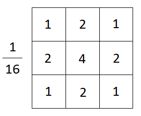
Traditional Gaussian filter kernel. Source:https://media.geeksforgeeks.org/wp-content/uploads/20201216123116/3x3GaussianKernel.png
In our network, there are different sets of weights for each convolution (of which there are 15 total) and each convolution has a different amount of in and out channels (160 in and 112 out at its peak) which also have their weights. So we have up to 160x112x3x3 (161,280) unique weights to use at one time. Luckily for us, this does not complicate the convolution code much, just makes executing it a bit more time-consuming. We iterate over the entire image using a different weight kernel for each channel, but we also have a different set for each output channel, which we then sum up.

Source: https://medium.com/swlh/a-comprehensive-guide-to-convolution-neural-network-86f931e55679
So for example at the start is a 4x32x3x3 kernel, where we apply a different 3x3 kernel to each of the 4 input channels from our image, and then sum up the resulting values to form one output channel value, we then do it 32 times total, taking the next set of weights each time and we have our new convolution output. One thing to mention is that the convolution should use zero-padding since we want to maintain resolution throughout the entire U-Net.
Weights
One thing I haven’t explained yet is where we get our weights from. Well observant reader, you are in luck, because as well as providing the source for their denoising neural network, Intel provides a set of float16 (and float32) weights to be used with it. Unluckily the header part of it is in a proprietary format, but is fairly simple to deconstruct with the source provided.
Optimizing
With all of the operations made, and weights parsed and loaded, we should now be able to denoise images at will, as long as our will is to wait 200 milliseconds for a 512x512 denoised image. The neural network is made up of 43 individual steps, but with a bit of profiling it seems that Convolutions take up most of the time (a whopping 97.7% of total time), which is of no surprise because we are doing a couple hundred million operations per convolution operation and that does not include the IO of loading the weights or input image.
Early exits
Since we are doing a convolution in 4 dimensions, we end up doing a lot of looping, where some of those end up being outside the input image and we pad with a zero value. However, since we are summing up the results, we can simply skip the current loop, as adding 0 and simply skipping the add yields the same result.
Preloading input and weights into shared memory
Another thing to consider is that since we are using convolutions to go over a 3x3 area of the image, some of our input pixels might get read multiple times (up to 9x), which if we are accessing them from global GPU memory is slower than it needs to be. So to fix that we load an 18x18 tile of inputs (16x16 but we also need neighbors for the convolution) into shared memory for one input channel at a time, and convolve over that (which is 7.1x less global reads). For our weights, since they are also shared for the channel, we can do the same so we don’t have to read them per thread.
Removing branching
Earlier I mentioned that we can simply early exit a loop if we find ourselves outside the image, but branching on the GPU can be expensive at times and in our case replacing the branching, and multiplying our weighed result by the condition of the if statement instead, we save ourselves 16ms.
Implementation in the breda-nn framework
Luckily for me, I didn’t have to implement any of the neural network foundation code, just the compute shaders, their “operations” and the U-Net itself. I was provided with a framework for creating neural networks, which was very easy to use once you started to understand how they work.
I could simply create a new Operation by implementing the respective rust trait and then creating functions for the shape of data we’re inputting, outputting, and which shaders to execute.
impl Operation for Upsample2D {
    fn create_inference_resources(
        &self,
        input_shape: &Shape,
        persistent_store: &mut RenderGraphPersistentStore,
    ) -> OperationResources {
        OperationResources {
            input_shape: *input_shape,
            auxiliary: vec![],
            output: Tensor::empty(
                "upsample2D_forward_output",
                self.output_shape(input_shape),
                false,
                persistent_store,
            ),
        }
    }

    fn inference_forward(
        &self,
        input: &[&Tensor],
        resources: &OperationResources,
        _parameters: &[Tensor],
        shader_db: &dyn ShaderDatabase,
        render_graph: &mut RenderGraph,
    ) {
        let input = input[0];
        let forward_output = &resources.output;

        let dispatch_size = resources.input_shape.w * resources.input_shape.h;

        let constants = [
            forward_output.shape().w,
            forward_output.shape().h,
            forward_output.shape().c,
        ];

        ComputePass::new("upsample2d-forward", render_graph)
            .constants_buffer(&constants)
            .read(input)
            .write(forward_output)
            .dispatch(
                &shader_db.get_pipeline("upsample2d-forward"),
                dispatch_size.div_ceil(GROUP_SIZE),
                1,
                1,
            );
    }

    fn create_training_resources(...) -> OperationResources {...}

    fn create_trainable_parameters(...) -> Vec<Tensor> {...}

    fn training_forward(...) {...}

    fn training_backward(...) {...}
}
Once I implemented each operation (pooling/upsampling/convolution) I could then create an operation that encompassed all of the aforementioned ones, executed in the right order, and the input/output shapes being passed through so each operation automatically gets resized to the correct size.
I think that without this neural network foundation, and some very handy built-in support for comparing our results with PyTorch by loading and running ONNX models exported from PyTorch directly in breda-nn, it would’ve taken me way longer to get this up and running.
info!("upsample inference:");
run_onnx_inference_test(
    "./apps/breda-nn-test/assets/models/upsample_inference.onnx",
    &*shader_db,
    device.as_ref(),
);

info!("max pooling inference:");
run_onnx_inference_test(
    "./apps/breda-nn-test/assets/models/maxpool_inference.onnx",
    &*shader_db,
    device.as_ref(),
);
Test on G-Buffer data
OIDN also can enhance image denoising by utilizing auxiliary g-buffer data, including normals and albedo. This approach significantly improves the reconstruction quality compared to only supplying a noisy image.

OIDN input, from left to right: rendered image, normals, and albedo
The result below is from one of the examples shown on the OIDN website (Mazda scene by Evermotion) and denoised in our framework.
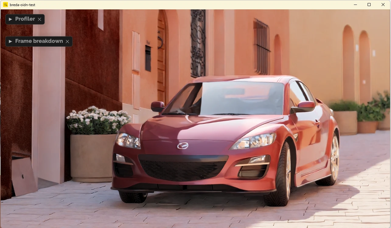
Denoised result running in real-time in our framework.
Conclusion
Overall I’d say that OIDN is an interesting bit of machine learning, and getting the opportunity to implement it has taught me a lot about neural networks and compute on GPU. I am happy with the result I’ve achieved, but in hindsight, I think I could’ve done better.
The internship at Traverse has been great, even at the interview, the people here were nice and welcoming. The atmosphere in the office is always great and asking for help and/or advice is easy and encouraged. The codebase is well structured and there's always someone ready to help out if you get stuck or are unsure about something. In conclusion, I’d say if you ever get the opportunity to be at Traverse, I wholeheartedly recommend it.
I’d also like to extend a special thanks to Max Liani for the articles about his journey implementing OIDN in his raytracer. They are well-written and were fundamental in my understanding of machine learning and OIDN.