

This blog post is aimed towards people with an interest in graphics who have knowledge about BRDFs and the math involved. In this post we will briefly go over how the layered material model we implemented works.
Layered material models are an expandable solution to achieve more complex visual appearances like coatings. The core idea is to combine multiple lobes by treating them as a stack of layers where light reflects off and refracts through. We based our implementation on the Weidlich-Wilkie material model, mainly to determine how layers interact with each other using simplifications from the paper to drastically reduce the computational complexity. For conductors we use measured data to get a more realistic approximation. We used three wavelengths to approximate the entire spectrum of light and use measured indices of refraction and extinction coefficients for our simplified Fresnel derivation. Simple BRDFs often hack conductors using Schlick’s Fresnel approximation with an eye-balled color that represents the conductor as F0.
Fresnel and our conductor model
We use two derivations of the Fresnel equations together with measured data for results closer to reality; one for dielectrics and one for conductors. For both derivations we assume unpolarized light, therefore the ratio of reflection and transmission depend on the average of p- and s-polarization of the incident ray. Since the per-wavelength varying extinction coefficient has a great impact on the visual appearance of conductors we use a slightly more complex derivation than we are using for dielectrics with an extinction coefficient factor. Since we are not working with a spectral renderer we had to pick frequencies to sample so we decided to go with three wavelengths to approximate the entire spectrum, 0.63 µm (red), 0.532 µm (green) and 0.465 µm (blue). The derivation to be used is selected based on the layer’s metallic factor, when this is zero it is a dielectric, otherwise it is treated as a conductor. Using metalness textures can lead to situations in which both derivations are linearly interpolated based on the metallic factor. Blending Fresnel for conductors and dielectrics is not physically plausible but is supported since it is often encountered in PBR assets and clamping or rounding the metallic factor would lead to loss of detail. Because we are approximating the entire spectrum with only three wavelengths, we use a lookup table with indices of refraction and extinction coefficients per wavelength for the following measured materials: aluminum, brass, copper, gold, iron, lead, mercury, platinum, *silver *and titanium. Our data set is obtained from https://refractiveindex.info/ of which we use the metal section of the 3D shelf.
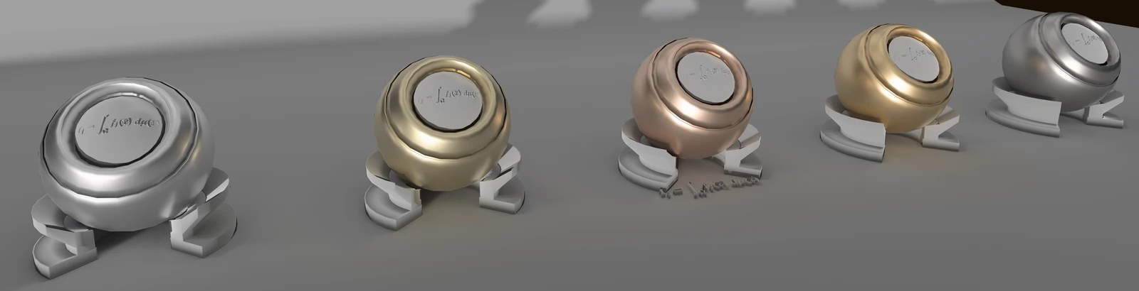
from left to right: Aluminum, brass, copper, gold and iron
For composing layered materials, we currently support GGX reflection, GGX transmission and Lambertian diffuse lobes. We support up to 4 components and enforce that conductors and diffuse lobes can only exist as bottom layer. Scattering within layers is ignored, and outgoing rays that encounter total internal reflection are invalidated. The invalidation of total internal reflection layers can cause energy loss, but this is compensated by an energy compensation factor.
Supported lobes
The Lambertian diffuse reflection lobe can only be used as bottom layer and represents an ideal diffuse material with a user specified base color. This layer represents a cheap approximation of scattering below the surface, causing the surface to look the same independently of the view direction. This layer only has a single base color parameter specifying the reflectance of the diffuse layer. This can be represented as a RGB color value or SRGB texture.
The GGX specular reflection lobe can be used to represent dielectric coatings on top of diffuse layers, but can also be used to model conductors. This is all determined by a metallic factor, which should either be zero or one. When metal-roughness maps upload values between zero and one it becomes a blend between dielectrics and conductors which is not physically plausible. We still support conductor dielectric blends in textures since it is commonly encountered in PBR metalness textures. Conductors in our layered model are assumed to not transmit energy since all energy is absorbed before it reaches the next layer.
The GGX specular transmission lobe is used to represent transparent materials, this adds a GGX lobe below the stack of layers. For indirect illumination we currently render the result of this lobe to a different texture since it cannot be handled by our indirect specular reflection denoiser in our hybrid renderer.
The layered BRDF
To sample the BRDF as a whole we sample a direction in all lobes individually and importance sample one based on a heuristic that determines which sample will likely have a high contribution. For diffuse lobes this returns the luminance of the diffuse albedo and the specular component will return the luminance of the Fresnel component. The heuristic for the Fresnel component can in the future be improved by taking the context of the layer into account, reducing the weight of samples from which a large fraction of incoming radiance has been absorbed by the layers above.
When a sample has been taken the probability density has to be calculated. Since a sample can be valid for all lobes, the total probability density needs to be calculated for the entire BRDF. When imagining a GGX specular reflection lobe on top of a Lambertian diffuse lobe, all samples taken on the GGX lobe are also valid for the diffuse lobe.
Re-using samples for all lobes makes our *sampleBrdf *and *brdfPdf *functions slightly more complex than when dealing with a single layer at a time. When we sample a BRDF we use random numbers to sample a direction in a lobe for each layer and a random number to sample one of the sampled directions that will be traced. Each sample will then get a weight assigned based on is luminance as mentioned before. A CDF is built using the weight for each layer and the third random number is used to sample one of these layers, only the sampled layer is traced. These weights are then normalized and sampled as CDF to determine which layer will be stored and traced.
The probability density* *function needs to account for the importance sampling of layers when calculating the probability density in order to converge to the correct result. This requires the *brdfPdf *function to be aware of the probability that the layer is sampled on the lobe. Since the sample can be valid for multiple lobes we multiply the sum of probability densities for sampling the sampled direction in each individual lobe by the probability density of sampling the lobe itself to get the total probability density that the direction is sampled. We validated our implementation by comparing the converged result to a result converged with next event estimation.

A shader ball with, from left to right, 2, 3 and 4 layers.
Calculating the reflectance of the BRDF consists out of several steps. We first calculate the reflectance of the top layer with given incoming and outgoing directions, then the absorption factor is calculated to attenuate the transmitted fraction of the incoming radiance. After that both the incoming and outgoing directions are refracted for the evaluation of the next layer. This uses Snell’s law with the index of refraction of the layer the light is refracted through. The total reflectance of all individual lobes summed results in the total reflectance of the BRDF.
Hopefully this post gave you some insight in how we tried to achieve more realistic layered materials by briefly going over our conductor model and by describing how separate components can be combined to achieve more complex results.