Dynamic diffuse global illumination

Code sample — see the original on Medium, linked at the end of this post.

This blogpost will cover how we set up our dynamic diffuse global illumination system in our rendering framework at Traverse Research. It’s completely ReSTIR based, but we won’t be focussing as much on how ReSTIR math works, instead we’ll focus more on the tricks, techniques and things we tried with setting up this system.

Performance breakdown

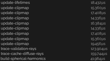
Timings were measured on an RTX 3080 running at a native resolution of 1440p while running the scene Flying world: Battle of the Trash god.

Camera position: [7.8699145, 2.2485592, -7.960048]
Camera look at position: [7.840394, 2.066986, -8.942983]

In total we use the following number of rays:

Indirect diffuse: 0.25 diffuse rays/pixel + 0.25 shadow rays/pixel + 0.25 validation rays/pixel
Irradiance cache: An upper bound of 65535 * (4 diffuse + 4 validation + 8 shadow rays)

Indirect diffuse: 1.97ms

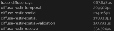
Denoiser: 697μs

Irradiance cache: 473μs

Candidate rays

For estimating indirect diffuse, we start off by tracing diffuse rays at half resolution. If we look at the ReSTIR GI paper, we should consider sampling the hemisphere uniformly rather than cosine-weighted. This will avoid low sampling probabilities on big lighting contributors at grazing angles, which can result in a much higher variance.

As for generating the diffuse rays, it’s generally a good idea to use blue noise. Though combining other noise techniques or combinations of them can also produce decent samples, if for example you want to abuse sampling patterns during spatial/temporal reuse or filtering.

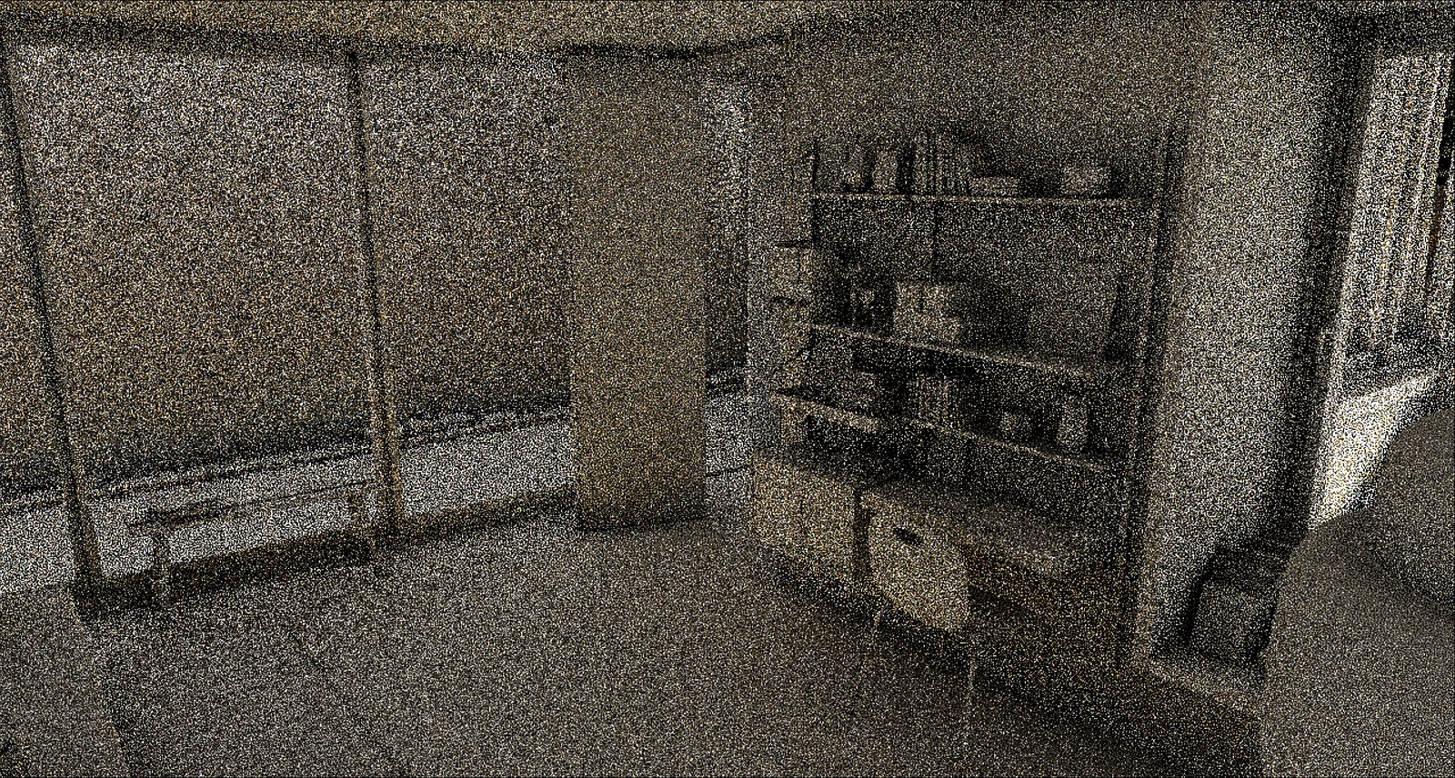
Blue noise generated candidates

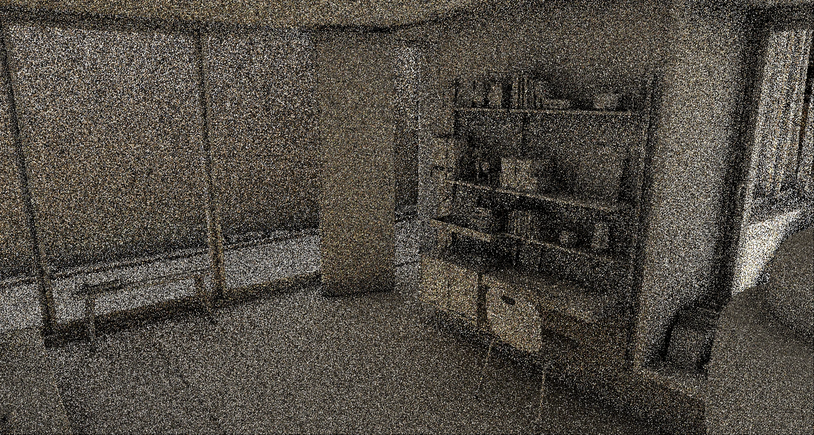
Blue noise + interleaved gradient noise generated candidates

If we’ve hit a surface, we sample the indirect lighting and direct lighting at the hit point. The indirect lighting comes from the irradiance cache in form of L1 spherical harmonics, while the direct lighting is estimated by tracing a shadow ray towards light sources.

Once we measured the incoming radiance from our candidate rays, we store the following information:

Sample direction
Hit distance
Incoming lighting
Sample hit surface normal

This may seem like a lot of data to store for each candidate, however we can compress this data down to a total of 4 uints. We encode the sample direction and hit normal as octahedron, for the incoming lighting we use R9G9B9E5_SHAREDEXP* *and finally we store the hit distance as full float.

NOTE: Since we are tracing rays uniformly over the hemisphere, we essentially get “free” ray-traced ambient occlusion, which may be useful to use in subsequent restir and denoising passes!

Temporal reuse

Temporal reuse is the pass where we need to be the most careful with sampling, reprojection needs to be accurate and rejection heurstics need to be relatively strict as all of our subsequent passes and frames rely on this pass. If our reprojected history is valid for reuse, we merge it with the candidate reservoir.

The output is still pretty noisy though as we clamp our reservoirs to a maximum sample count of 12.

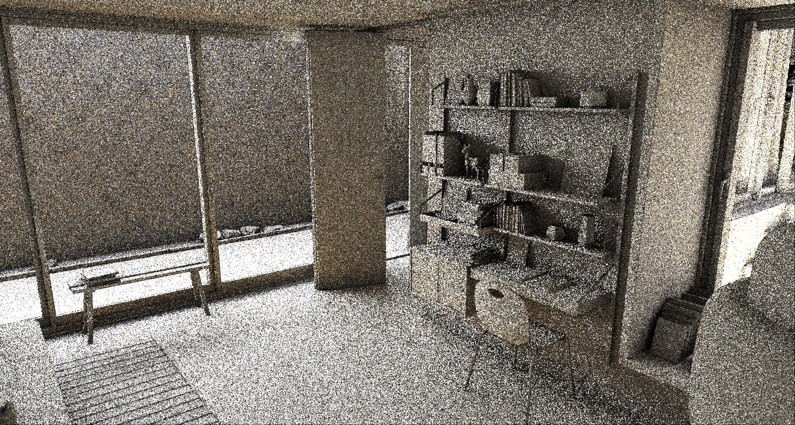
Temporal reuse

A technique that we can use to reduce variance further is permutation sampling, the idea is pretty simple; we use a global jitter and afterwards xor the reprojected pixel index by a value, which results in an ordered spatial exchange of history reservoirs.

This is kind of the same idea as running a spatial search in temporal reuse. However if we were to use naive spatial resampling here, we would get massive correlations between pixels as multiple pixels would be resampling the same neighbor reservoirs, resulting in “clumps” of bright samples. The most ideal pattern seems to be a global xor value that changes every frame in a range of [1..3], though a naive xor of 2 or 3 works fine as well.

We chose to gather multiple permutation samples each temporal reuse pass, while exponentially decreasing the sampled reservoir M clamp. While this does initially make the temporal reservoirs less accurate, it helps a lot with disocclusion. Detail is recovered by using guiding masks and ReSTIR validity frames. Alternatively you can also choose to only run a set of permutation samples when the center reservoir is starved for samples (for example a newly disoccluded pixel).

Since the permutation samples came from a different origin we must make sure that we apply a jacobian here.

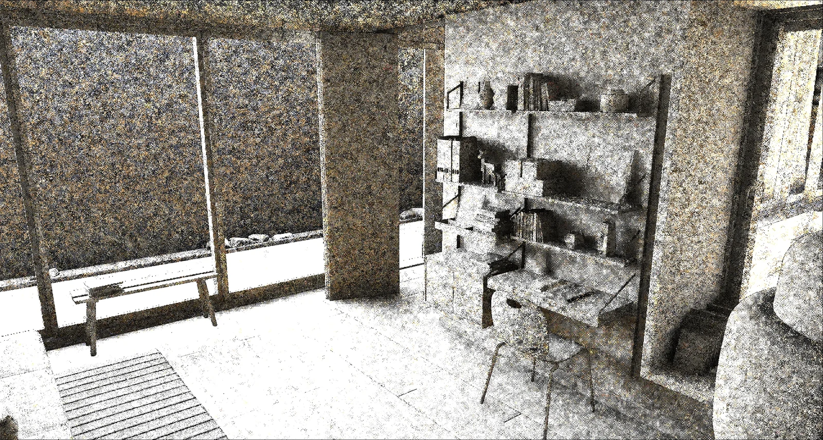
Permutation sampling

We don’t know if the merged reservoirs had a visible sample, naively merging these reservoirs in this case results in loss of contact shadows. The correct way of preventing this would be to simply trace the visibility of these samples, but this is too expensive as we have a very limited ray budget. Instead we can use an indirect shadow guiding factor generated by the previous frame, and reject permutation samples if their “shadow” values differ too much, more on this in the spatial reuse section.

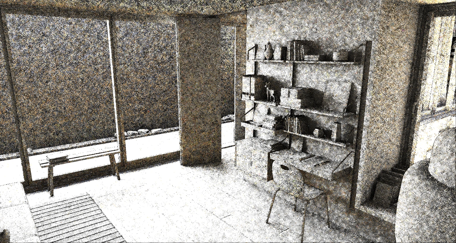
Permutation sampling with indirect shadow guiding

Smaller details and shadows are better preserved temporally with indirect shadow guiding. Not being careful here can result in much more visible disocclusion/movement artifacts in dynamic scenes, which are very difficult to filter.

As for guiding/rejection techniques we’ve tried to use an average sampling direction from the selected reservoirs, SSAO masks or even denoise the RTAO we got for free earlier on. All of which have their advantages and disadvantages.

There may be other ways of steering sampling/rejecting samples, visualizing specific sampling data produced by resampling may give some ideas on what you can (ab)use to refine rejection heuristics!

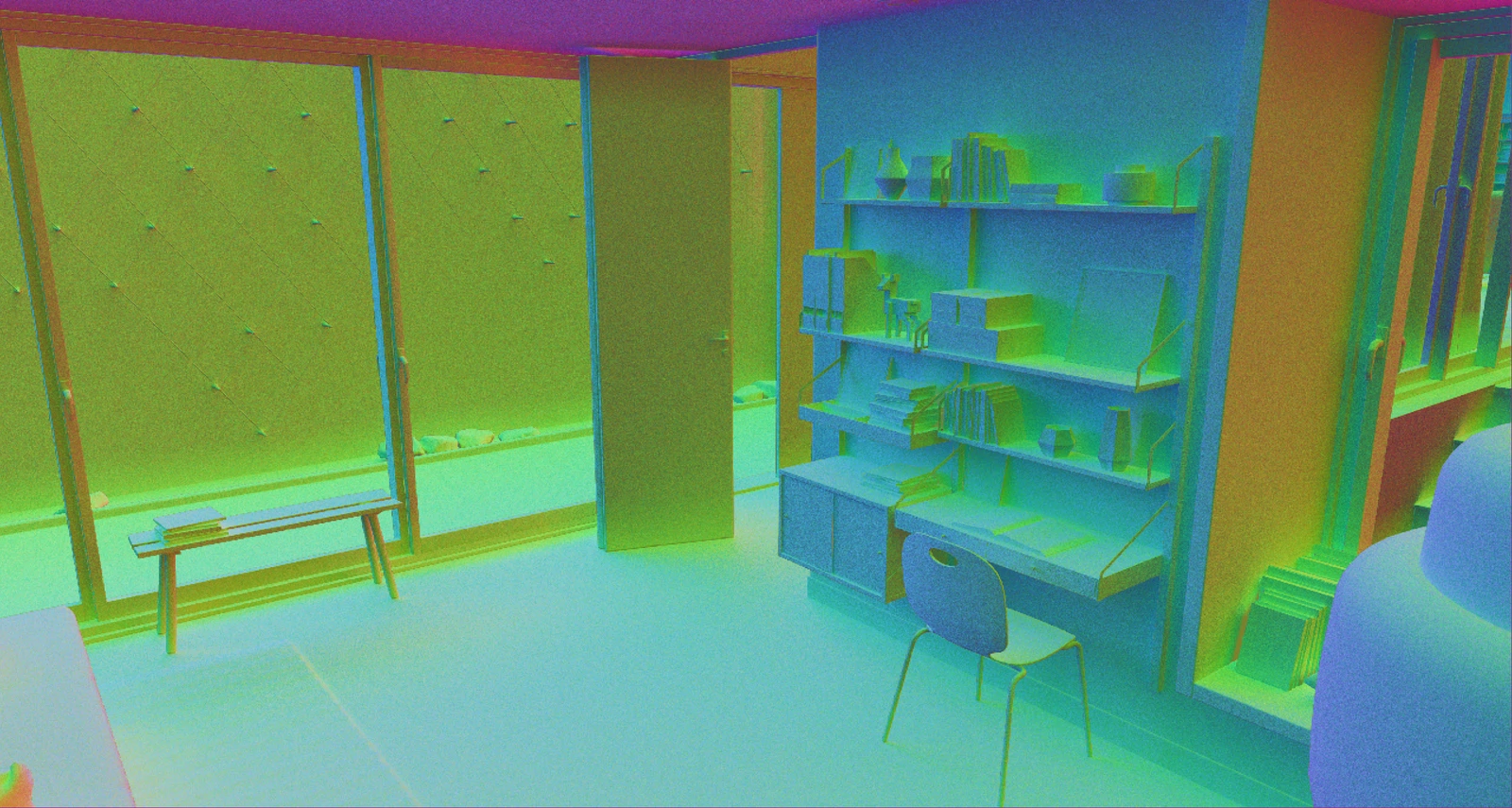
Average reservoir sampling direction visualized

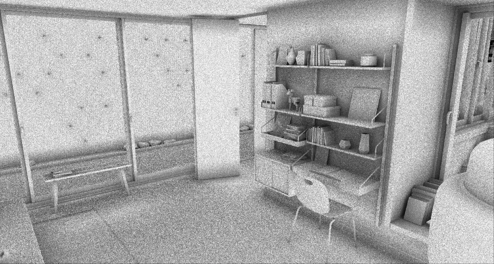
Reservoir W visualized

Spatial reuse

For spatial reuse we run two separate kernels, the first kernel does a large spatial search with a radius around 4% (42 pixels) of the rendering resolution. The second kernel runs the same logic but instead takes less samples and runs at roughly 2%(20 pixels) of the rendering resolution, though this can be smaller depending on how low the sample count of the center reservoir is.

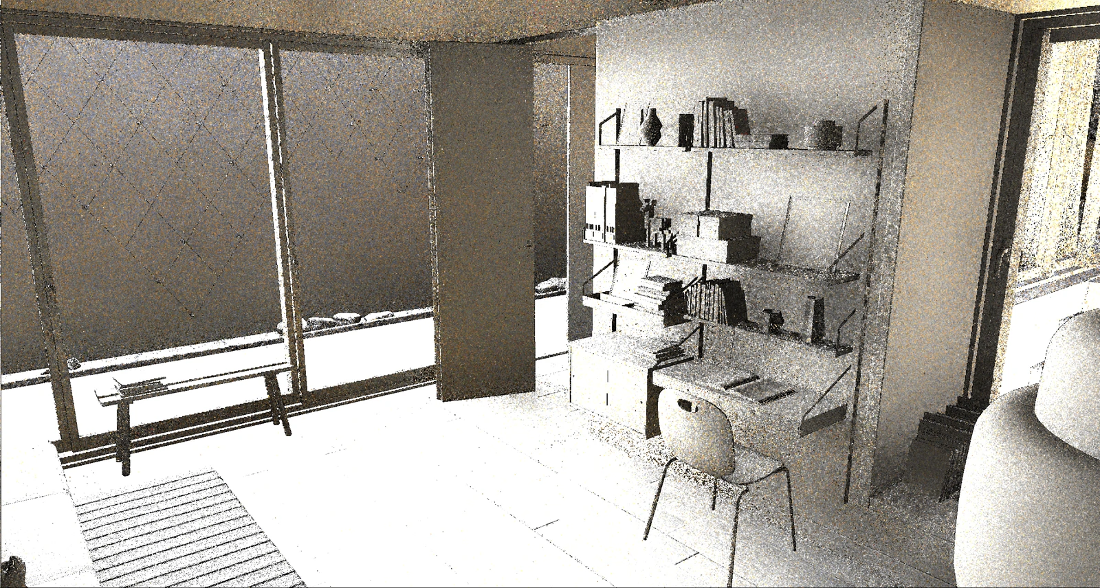
ReSTIR spatial reuse result

Both these spatial reuse passes don’t do anything fancy besides merging reservoirs that survive the rejection heuristics. In order to reject “bad” reservoirs, we compare normals and measure the tangent plane distance between the center and picked reservoirs. Finally we also apply the jacobian, if the reservoir has survived these checks and does not have a rediculous jacobian, we go ahead and merge the picked reservoir.

Using the tangent plane distance here is essential to avoid excessively rejecting neighbor samples. When only using depth rejection, we tend to get a lot of “boiling” noise on surfaces that have a grazing angle with respect to the view point.

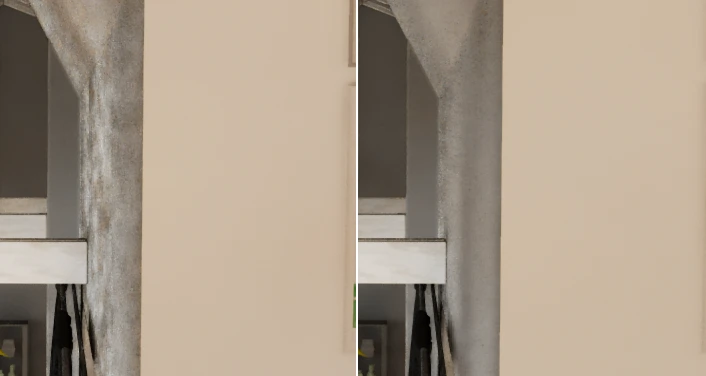
Left: Naive depth rejection. Right: Tangent plane distance.

So what happened to all the indirect shadows and details? We do not use guiding masks here to reject reservoir reuse, nor do we test visibility for each reused reservoir. Testing visibility for each reuse candidate is way too expensive if we were to use ray tracing as we would need to trace an additional 10–15 rays per pixel, though there have been some alternatives using screen-space ray marching.

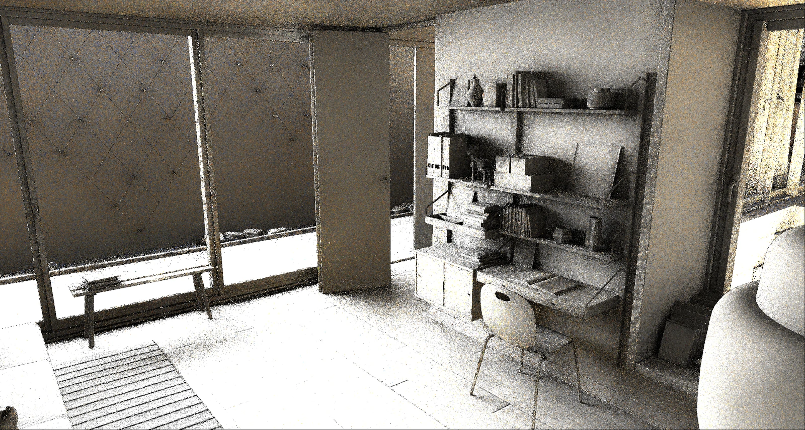
Testing visibility for each spatial reuse candidate

Instead we keep the spatial reuse simple and light-weight. Afterwards we only test visibility for the final surviving reservoir. If the sample is occluded, the result sample will simply have 0 contribution. This is obviously biased and introduces some noise, but in reality provides a nice tradeoff between quality and performance.

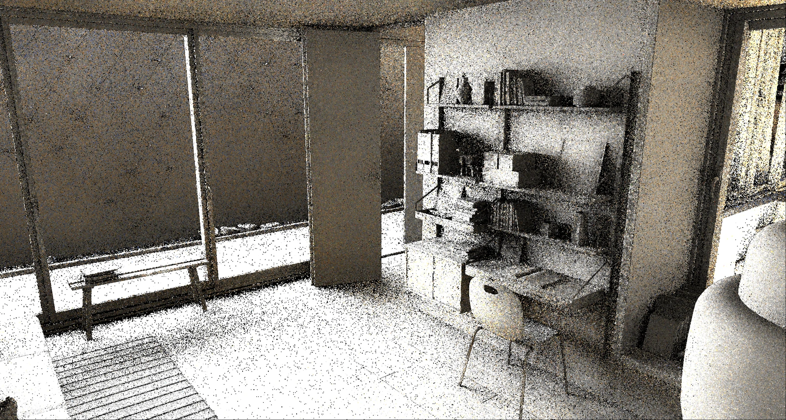
Testing visibility for the final surviving reservoir after spatial reuse

Now that we’ve tested the visibility of all of the surviving reservoirs, which tend to be specifically towards indirect light sources with the highest contribution, we may find the results of these visibility tests to be useful for more than just validating reservoir visibility. Let’s see what this actually looks like if we were to treat it like a shadow mask:

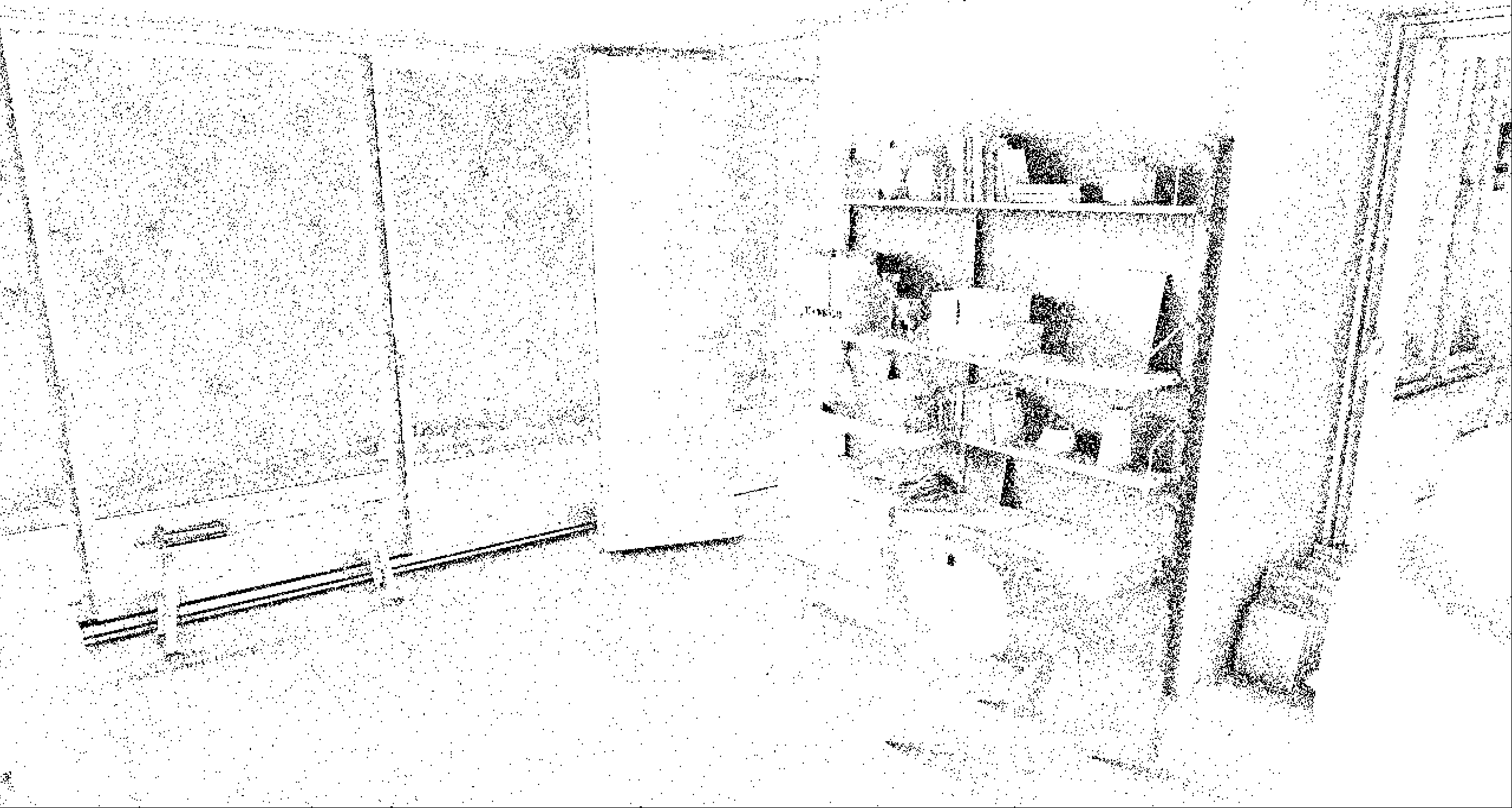
Treating final visibility traces as a shadow mask

This seems to exactly mark the regions where we would need to be extra careful with spatial exchanges and filtering! We definitely don’t want to “smear” out our indirect shadows in subsequent passes and frames, now we can just measure the shadowing difference between pixels and reject based on that.

Ideally we would have a denoised version of these indirect shadows:

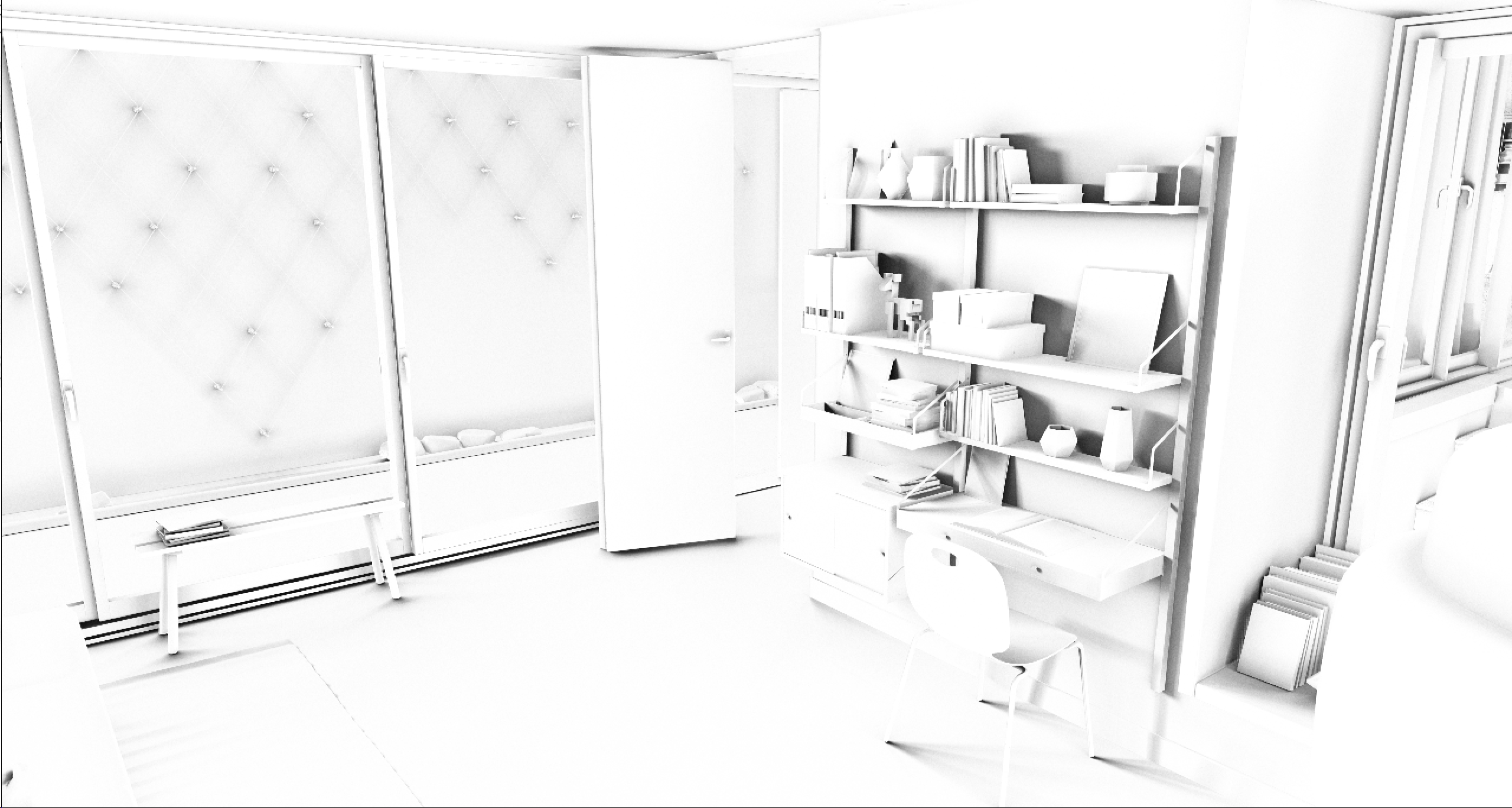
Accumulated indirect shadows

However doing an extremely cheap spatio-temporal blur with adding some bias towards shadow hits that have a shallow angle actually appears to be more than enough. We only care about the difference between pixels rather than actually modulating the final indirect lighting.

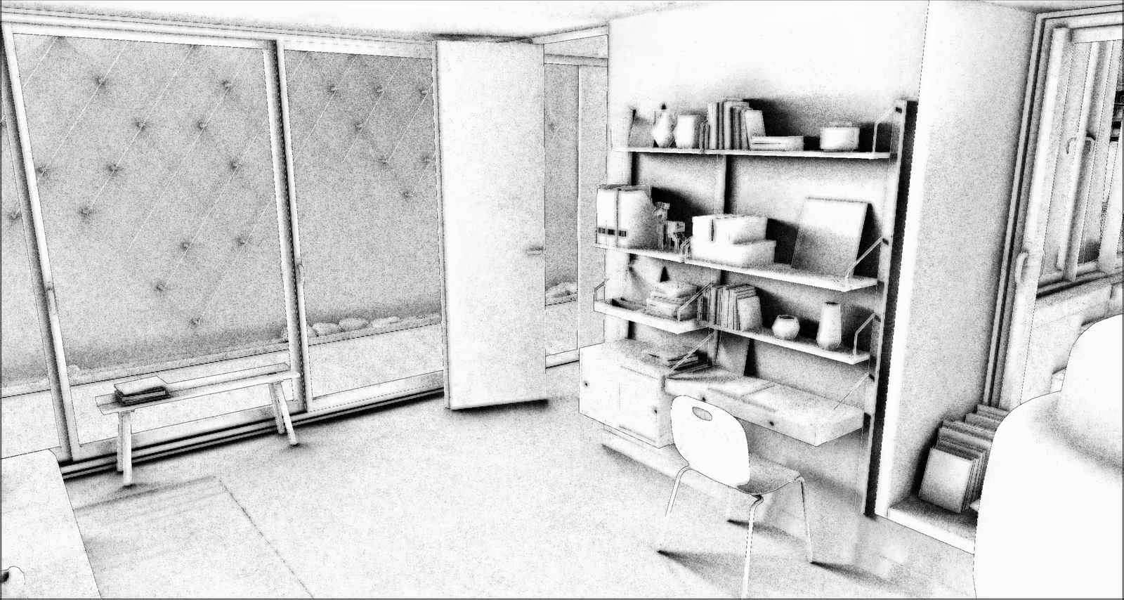
“Denoised” indirect shadow guiding factor

Additionally, in the future we’d like to explore this idea and try storing the occluded direction instead. Doing so might prove useful as a way to estimate visibility during resampling. This way we can be more specific on what samples get shared rather than only comparing their indirect shadow factor.

Consider the following situation:

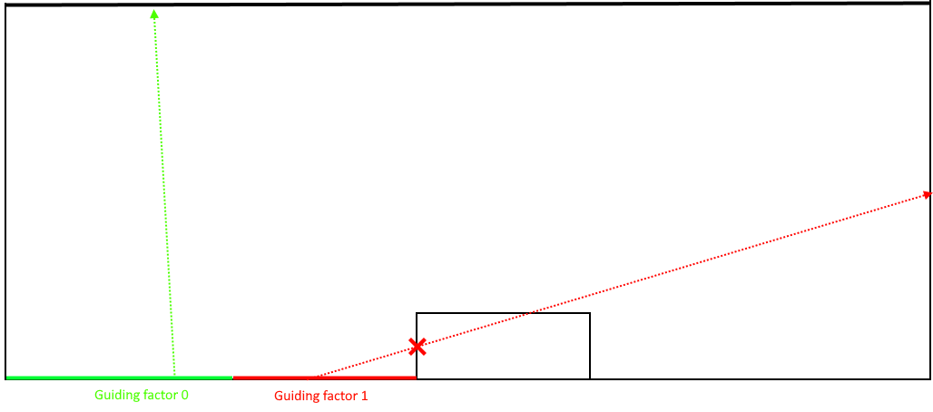
Green had a visible sample and has a guiding factor of 0, red had its final sample occluded and now has a guiding factor of 1.

In this scenario we would reject sharing reservoirs between green and red, as their guiding factor differs too much. This is a problem since the green sample is actually visible from the red marked surface.

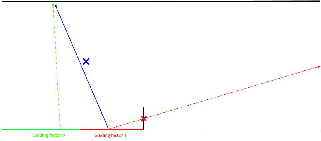
We reject potential reuse from the red origin marked with the blue line

If we were to make the guiding factor consider directionality here, we would still reject any samples that would roughly come from the occluded direction, while being able to reuse samples that are more likely to be visible from other directions.

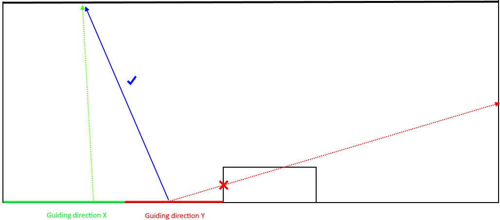
With directionality, we could potentially reuse the green sample from the red surface, indicated with the blue line

Resolving to full resolution

Now that we have validated our reservoirs after spatial reuse, we can resolve them to full resolution. We do this by taking 4 samples per pixel in a small screenspace radius. Furthermore we reject samples that differ too much in the indirect shadowing factor, this helps to preserve sharp indirect shadows.

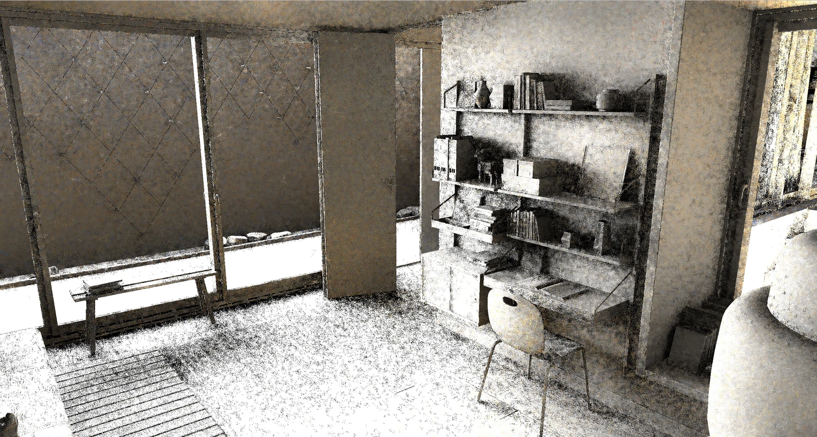
Resolved reservoirs with only testing visibility for the final sample

We observe quite a lot of noise still being present here, which is the result of us being cheap about testing visibility. If we compare this to the resolved reservoirs that actually had all their visibility traced during the spatial exchange passes, we may be able to be less aggressive during denoising, however we decided that the additional cost of tracing many more shadow rays is not worth it.

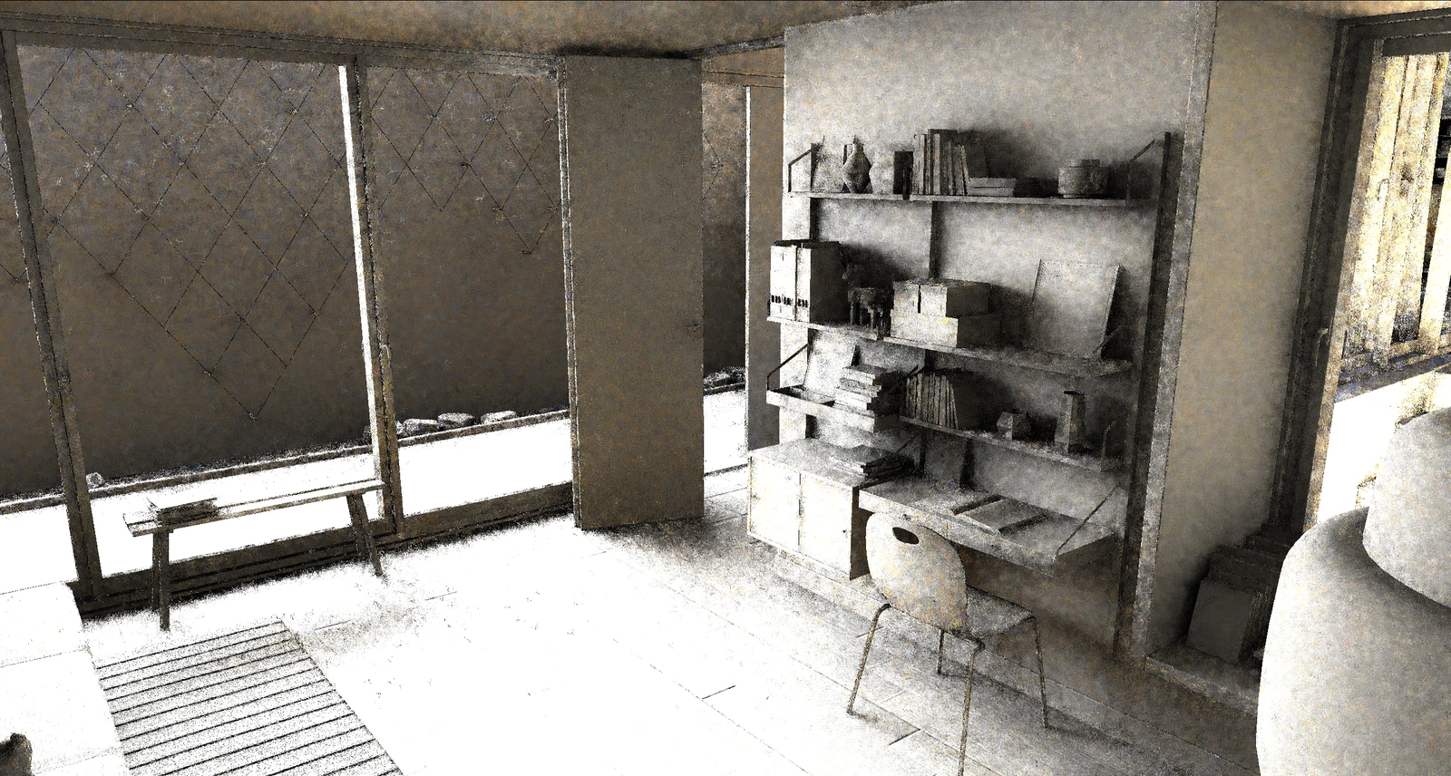
Resolved reservoirs with tested visibility during spatial exchange

For denoising we use a very basic spatio-temporal filter. We initially tried filtering in YCbCr here, but this gave some undesired “boiling” artifacts in the indirect shadow regions. Instead we we decide to use AABB color clipping to avoid hue shifts when lighting condition changes. Doing so resulted in much more stable indirect shadows.

Once again we use the indirect shadow guiding mask here to manipulate the accumulation rate and history rejection; indirect shadows from occluded visibility rays tend to be significantly more noisy compared to those which were not occluded, we accumulate at different rates based on those properties. If the indirect shadow factor shows a very large change, the accumulation rate gets changed accordingly to be more reactive.

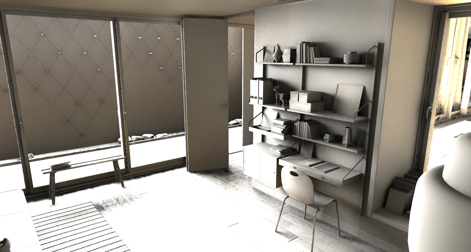
Temporal reprojection

Most remaining noise is then cleaned up with a small bilateral filter.

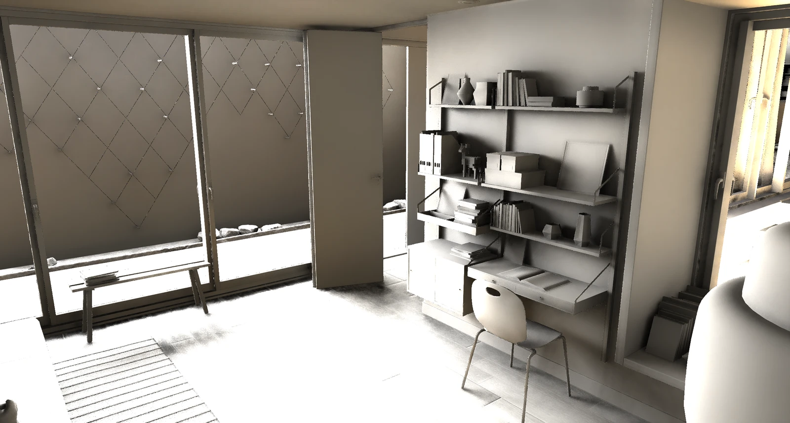
Final cleanup

Once we have the denoised indirect lighting, we simply modulate it with the albedo, let TAA take care of any remaining noise and we’re done!

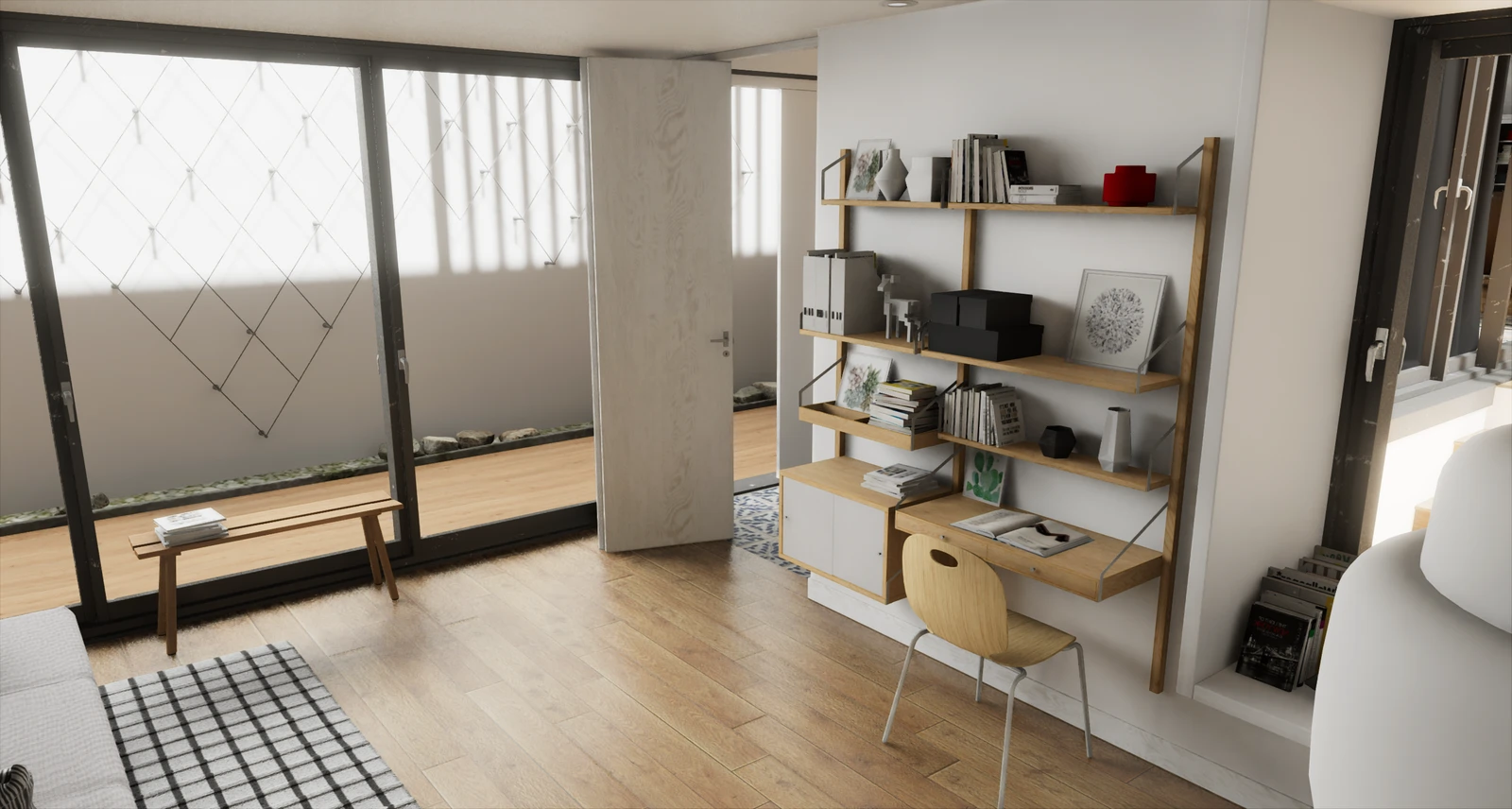
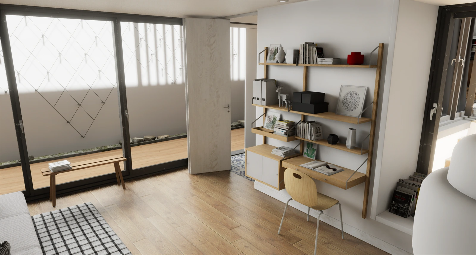
Final output

A quick note on handling alpha tested geometry, we found that masking out alpha tested materials for all the diffuse traces, and enabling alpha testing for the final visibility test produced the best quality vs performance. Limiting the number of alpha tests a ray can evaluate may help with performance.

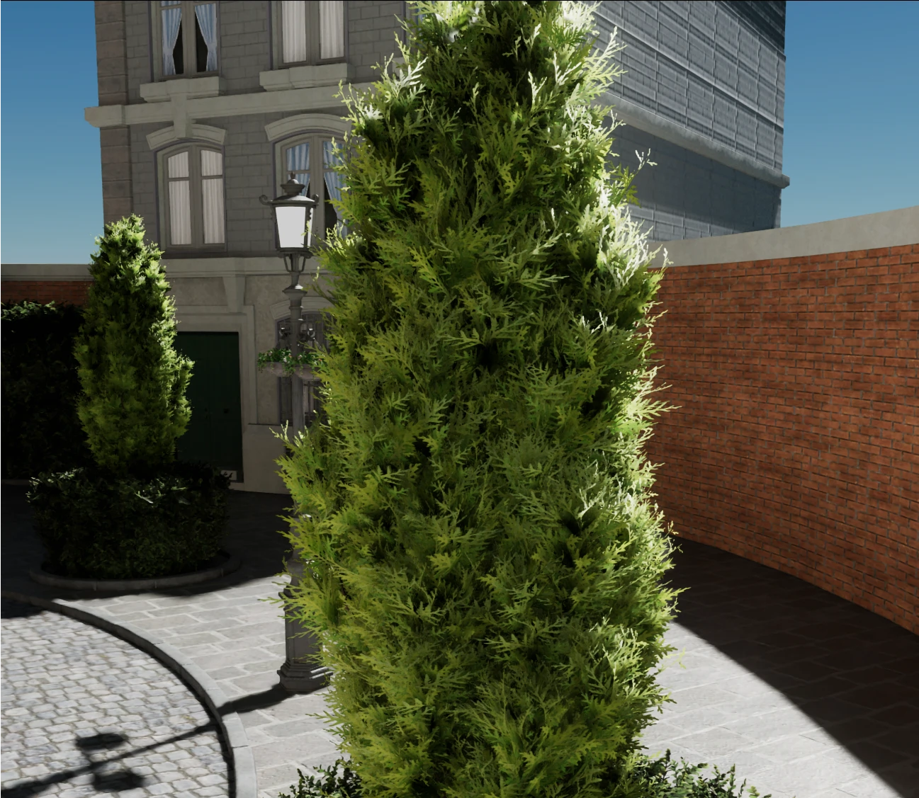
Test alpha in diffuse trace + test alpha in final visibility trace

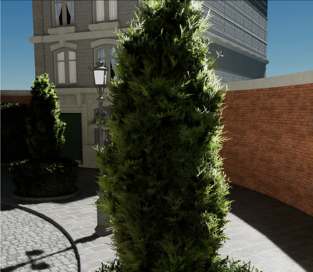
Force opaque in diffuse trace + test alpha in final visibility trace

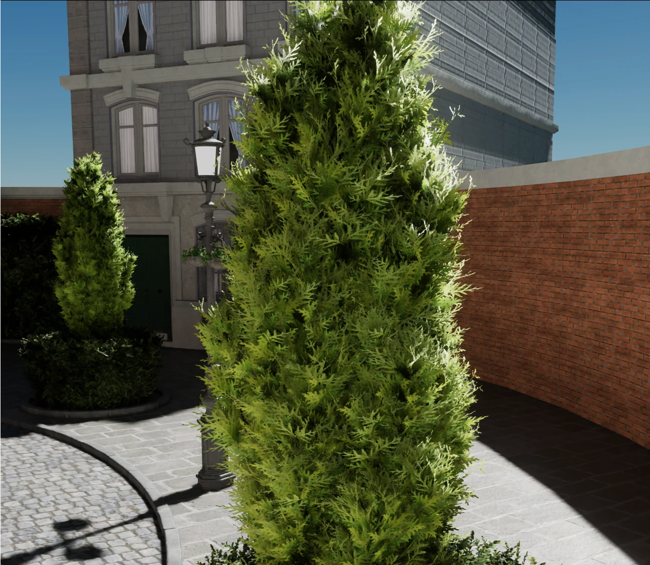
Mask out alpha in diffuse trace + test alpha in visibility trace

ReSTIR validation

To keep the scene responsive to light changes, once every three frames a ReSTIR validation frame is executed to re-measure the selected reservoir’s data. If the hit position or incoming radiance of the sample is different, we scale the reservoir M down accordingly. This will make the indirect diffuse reservoirs much more responsive.

However if we would *only *trace validation rays during such a validation frame, newly disoccluded pixels would not get traced at all. More importantly we would be wasting validation on pixels that possibly have gone off-screen. To solve this issue, we create a split in the tracing kernel. We start by reprojecting the history pixel location to the current frame, if the reprojected pixel location falls outside of the current screen bounds, we simply trace regular diffuse rays for that pixel, otherwise we proceed with tracing validation rays, as we have a history available that will be re-used in the current frame.

Irradiance cache

To estimate “infinite” bounces we will need a world-space irradiance cache that can be queried from any point in our rendering pipeline. Initially we went for a clipmap that holds an indirection to the underlying data. The clipmap irradiance cache is largely inspired by the irradiance cache used in kajiya, with some minor differences.

To give a quick recap: each entry in the irradiance cache places a probe at some distance away from its initial hit position. The probe is represented as a 4x4 octahedron map, where 4 diffuse rays, 4 validation rays and 8 shadow rays total are being traced from every single frame. Each ray samples the irradiance cache that it’s constructing, which leads to infinite bounces.

As an experiment we tried using a very lossy but cheap way to approximate shadow rays for all rays that query an irradiance cache entry. We did this by tracing a single shadow ray per irradiance cache entry and use use this result for all rays that would query it. This way we hoped to get around tracing additional shadow rays towards light sources from our diffuse bounces, but turned out to be extremely biased as we now mark the entire cache entry as lit or unlit. In the end it really was not worth it at all as we would only be tracing a relatively small amount of shadow rays less per frame in total, while getting significantly less accurate indirect lighting.

For each entry in the 4x4 octahedron map we store the same information as our diffuse candidate rays:

Incoming radiance
Reservoir
Sample direction
Hit distance

Just like in our indirect diffuse kernel, all of this info is again compressed the same way to a total of 4x4x4 uints per cache entry.

After tracing all the candidate rays, we apply temporal reuse to keep track of the most important samples. During each frame we also select 4 reservoirs to perform ReSTIR validation on, these reservoirs are the most frames away from getting new candidate samples. In a 4x4 octahedron map, this would be the set of samples of frame index *(currentFrameIdx + numberOfTraceFrames / 2) % numberOfTraceFrames where numberOfTraceFrames *is 4.

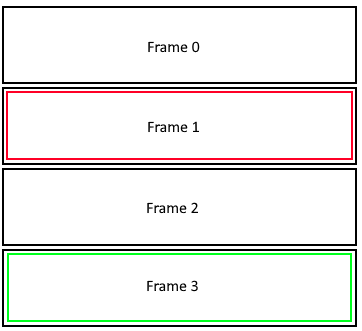
Diffuse candidate rays highlighted in green. Validation rays highlighed in red.

Let’s assume we are at frame 3, in the upcoming frame we would provide new diffuse candidates for frame 0. In the previous frame we provided diffuse candidates for frame 2, which means that the last frame to receive any updates is frame 1. This way we keep all of the 16 samples in our entry from not being stale for longer than 1 frame total.

Once we are done tracing the diffuse and validation rays, we build the spherical harmonics of the cache entry out of all valid samples.

For sampling the irradiance cache, we only have to load a packed L1 spherical harmonic, which is stored in a compressed format of 128 bits. Alternatively if bandwidth is an issue, you can also choose to go for YCoCg spherical harmonics which can be compressed to 96 bits.

Irradiance cache visualized

You may notice the irradiance cache entries are “wobbly”, this is not an artistic choice but actually has some purpose behind it. Imagine the following situation:

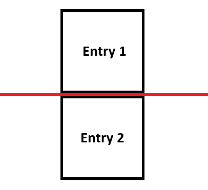
Two irradiance cache entries located at exactly the same distance to a vertex

When multiple irradiance cache entries are located at exactly the same distance to a vertex(red), which entry will we get when we query the position of the geometry? The answer to this question is yes..

Issue visualized

To get around this issue we can modify the lookup function of our cache entry by applying a periodic shift. What this does is drastically minimize the size of intersections between a given triangle and cache entries.

Same scenario but we apply a periodic shift in our cache lookup

There are problems with naively running a clipmap irradiance cache, one of the major ones being light leaking. There’s nothing stopping a ray from both the front and back of a surface from querying the same irradiance.

A good solution to this issue is a ranking system, which assigns a rank to the ray that queries the irradiance cache at a given position. Rays that originate from the screen have a ranking score of 1. Irradiance cache entries that were allocated with this rank will trace rays with a ranking score of 2 etc. New tracing origins will only be considered if the voting ray has an equal or lower score compared to the rank the entry currently has.

Let’s take a closer look at the scenarios where these light leaks happen though, we can observe that they mainly appear on places where the ray towards the query position is smaller than the size of a cache entry.

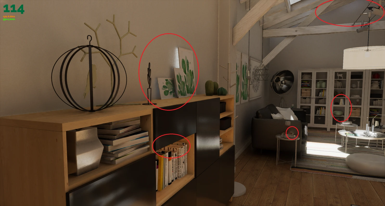
Light leaking by incorrectly sampling

As an experiment, we tried to just reject queries that meet this condition to see if this would be sufficient as well. This way we can let the indirect diffuse ReSTIR samples prioritise light that comes in from an angle that would exit the enclosed area, as the weight of those close hits would be 0.

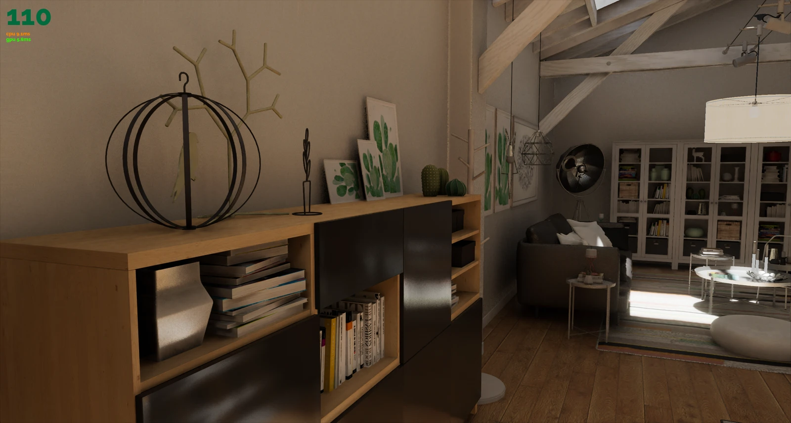
Light leaks gone by rejecting queries from hit distances smaller than a cache entry

Looking at the results we notice quite a bit of darkening happening in several locations, where light otherwise would be bouncing around. This works around the light leaking problem decently, but still would not stop location votes from ending up outside of the geometry.

Future work

Visibility caching

One of the “holy grails” of ReSTIR would be to efficiently cache and estimate visibility so we would not have to explicitly trace shadow rays for somewhat reliable resampling, DDGI does something along those lines with radial gaussian depth but lacks directionality which is essential for sample visibility.

Visibility bitmasks sounds promising if we could somehow convert them into spherical bitmasks and/or store a bit more information besides boolean visibility information, but this quickly would consume more memory than we might hope for. Additionally updating visibility with canonical rays may not be ideal; let’s assume we were to use spherical bitmasks at a resolution of 16×16 slices, we would need to test 256 directions to fully fill in the visibility mask. Perhaps using “spherical visibility masks” per N×N region of pixels might speed things up.

Denoising

Ideally we want resolve the reservoirs to spherical harmonics, and interpolate them to full resolution after the spatio-temporal denoiser in a separate pass. This should in theory greatly reduce blurriness in the final output, especially when the scene has aggressive normal mapping or geometric complexity. This might also allow for running the tracing and reuse passes at an even lower resolution, as interpolating the coefficients is trivial.

Irradiance cache

A clipmap irradiance cache works great, but quickly runs into memory footprint issues when trying to use a higher resolution. The main reason for this is that we store indices in a 3D texture, which wastes a lot of memory on empty space.

As an alternative, a GPU hash grid can be used as this opens up more potential for higher resolution irradiance/DI/path caches.

Hopefully this post gave you a bit more insight on what techniques and tradeoffs can be used when building a ReSTIR-based dynamic GI system. Trying to preserve micro detail while still keeping a clean and responsive image has proven to be extremely difficult without tracing an excessive amount of rays, but not completely impossible.

If you have any questions on specifics of this blog post that I did not cover, don’t hesitate to reach out on mastodon or X.

Finally I highly recommend checking out the links below as they provided all the foundations to build a dynamic GI system!