Let’s start with some general stuff first; this will be an introductory post about the Render Graph developed at Traverse Research, intended for people already falmiliar with the basics of GPU programming. The main concepts used are (render or compute) passes, (texture and buffer) resources, and barriers.
Additionally, back in April 2022 our dear Manon wrote a blog post about our render graph too! You can find it here. Compared to her post, one main thing has changed: we changed the way in which we group the passes. For those who haven’t read that post yet I’ll do a quick recap of the render graph. For those who have you can skip straight down to “Using the implicit chronological order”.
To start things off, I’ll reiterate something you’re already familiar with: we need to place barriers between our passes in order to execute the passes in the correct order and avoid race conditions between the resource reads and writes. Ideally, this number of barriers is as little as possible to reduce the total time we’re waiting.
🔍 Our in house renderer
At Traverse Research we have our own in-house renderer. This renderer creates many different kinds of passes in a plethora of different systems which all result in a single frame being rendered. Since we’re rendering a single frame, we want to dispatch our passes to the GPU in one single go. Furthermore, each of these systems doesn’t know what other systems exist and what passes they create, nor do we even want to be concerned with that. Ideally we can provide some sub-system with our inputs and get all of its outputs back and ready for us to use in any of our following passes. This means we can’t make some smart manual decisions about where to place our barriers.
♥️ Making our life easier and faster
So, we need some kind of way to tackle these issues. Let us start with the simplest: being able to give all our passes to the GPU at once. This can be achieved by creating a centralized place to which we can add our resources and passes. We’ll call this our Render Graph (you’ll understand the name at the end of this). Various other renderers have a similar concept, although the name may vary. With everything in a single place, I’ll leave it up for the reader to imagine how we can then pass everything to the GPU in a single go.
At this stage we aren’t doing any work on the GPU yet, so we aren’t limited by the limitations of a GPU just yet. We can still reason about any chronological ordering between our passes. However we also mentioned that when we call a sub-system, we just want to provide it some input and get some output resource back, without having to reason about all of the passes that the sub-system might be creating. Creating a chronological ordering between the passes themselves is thus off the table. So what do we actually have that we *can *use?
We can do both reads and writes to our resources. Reading does not change the actual data of said resource, but we can safely assume writing always will (otherwise why are you saying you’re going to write to it?). What we can do is adding a version number to each resource. When we read a resource in a pass, we explicitly state which version we would like to read. When writing to a resource we do everything as we would for reading the resource, but afterwards we increment the version, after all this is now different data! Any passes using the resource afterwards will use the now incremented version number. As a more real-world example: we have a canvas on which we painted yesterday and we’re going to paint on it again today. That means tomorrow it’ll also be different than how we started today. Whilst what we have painted on the canvas is different throughout the three days (version 1, 2 and 3), the actual frame and cloth of the canvas stayed the same.
By adding these version numbers to our resources, each of the passes have specific versioned resource dependencies. These dependencies implicitly describe the ordering that we will need for all of our passes! If you’re not directly following: the dependencies can be followed to link the passes to one another. To know what passes need to be executed before a specific pass, we look at all of its versioned resources used and for each resource find the pass that did the actual version increment. If we were to look at all of our passes from a global overview, we could see that our passes form a large graph network, hence the name Render Graph.
In our graph, the starting and ending points are always resources. When a resource is created it’s version number is 0, even when no data is passed to initialise the buffer with. A pass filling this uninitialized resource is still writing to it and thus incrementing the version number. At the other end of our graph we also end up with some output resource, after all adding resources that only read but don’t output anything themselves don’t do much for our render.
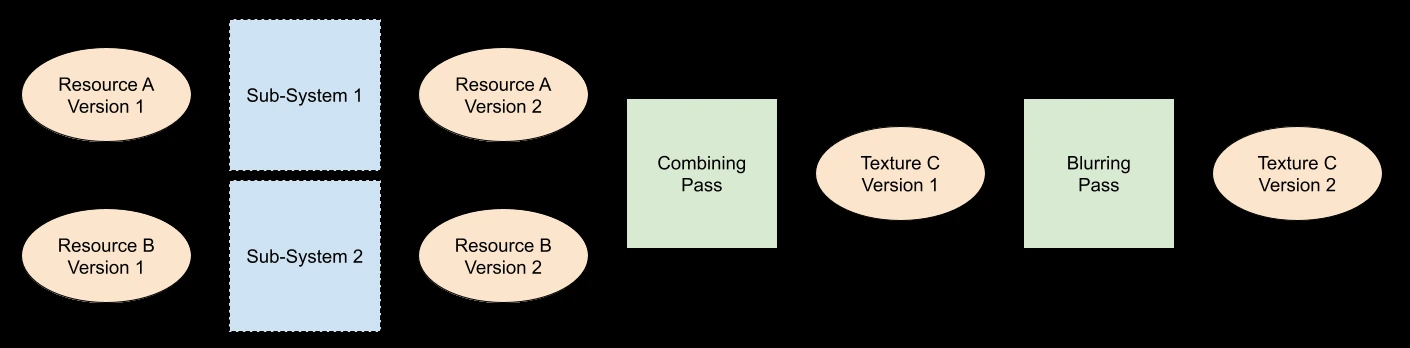
To make things a bit more visual, let’s look at a simple case. We have got two separate systems creating some output texture. These textures are combined in a new pass, after which the output texture is blurred. This will give us the following graph:
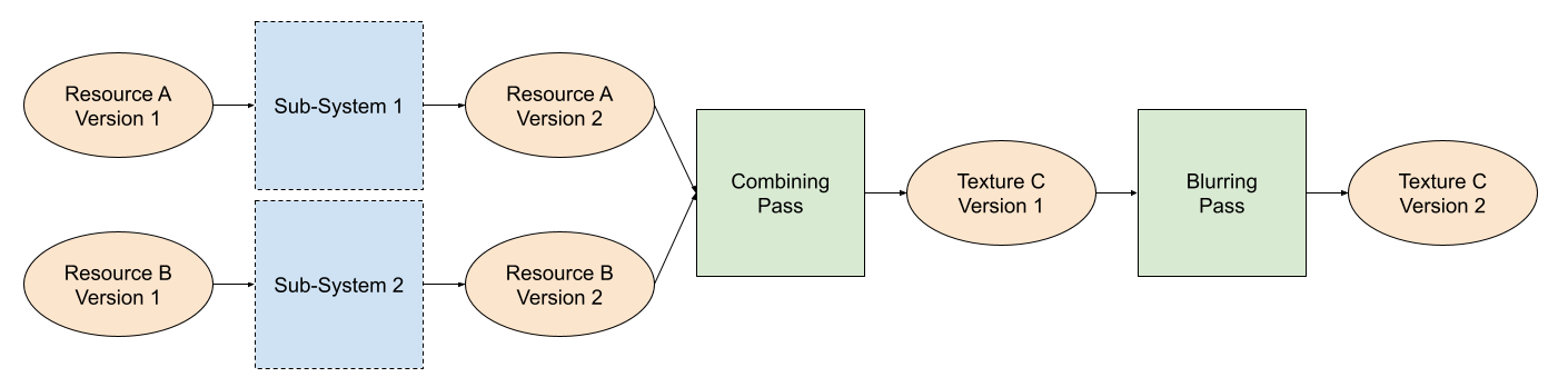
Partial Render Graph of our blurring pass
Just as a small note: this graph cannot contain “loops”; a situation in which we can follow any number of arrows and end up at the same location. This is the same for any system interacting with a GPU that does not contain race conditions. The official term for our graph is a Directed Acyclic Graph (DAG).
🏭 Using the implicit chronological order
We’ve got a graph with implicit dependencies, but where to place the barriers between our passes? We’ve mentioned that our initial knowledge of our Render Graph is mainly about the resources and their versions. For now we’ll assume each resource can truly only be written to by a single pass, i.e. there’s only a single pass doing a write operation to a specific resource and version combination. For the usage of a versioned resource, we can identify a few different cases: it’s only read by one or more passes, it’s only written to by one pass, and it’s read by one or more passes and written by one pass.
In all three cases we need to place a barrier between the pass doing the version increment and the passes using the version incremented resource. For the first and second cases there’s really not much more to do. The third one, however, has a small caveat: if we would use the same barrier for the reads as we would for the write, the write could happen before (or at the same time, being a race condition) the read operations, invalidating the data we expected to be there for the read. Thus, we need to make sure any read operations happen before any write operations. This can probably be solved in multiple ways, but we opted in our implementation to add an “invisible” dependency link from the reading passes to the writing pass. Let’s look at a visual example:
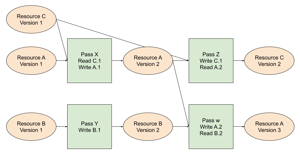
Partial Render Graph with more passes without barriers
In this example I have labelled each pass with what resources are used as input, as well as their usage and version. If I am not mistaken, the graph covers all different cases. Adding barriers to it would result in the following:
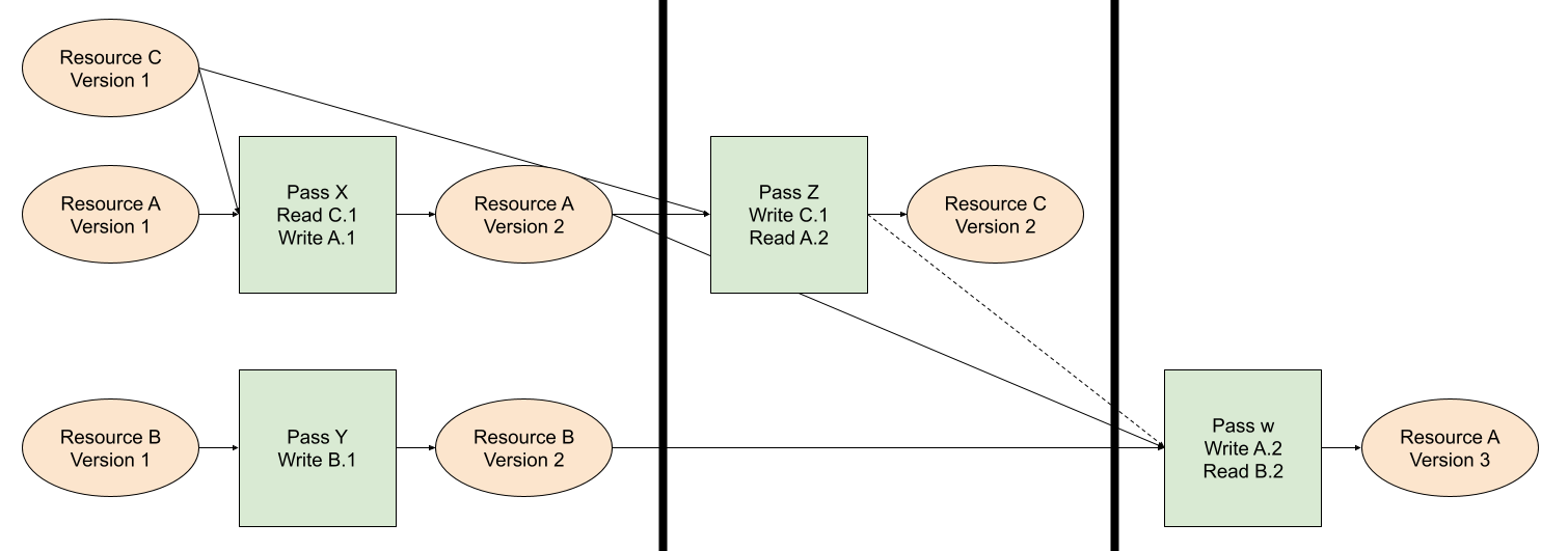
Partial Render Graph with more passes with barriers
Another way of looking at this is that we’re slicing the render graph into groups, where each group contains one or more passes which can be executed in any order (or all at the same time) without barriers.
🧑💻 Translating logic to an algorithm
In our system there are various code paths that do generate passes, but turn out to be unused for the actual output, these are mostly alternative (debugging) versions of the main render output. We do know which output we want for this frame, but we do not immediately know which passes become unused. Removing these unused passes is what we call dead stripping. The versioned resource which must be executed we’ll call root resources.
If we were to start at the beginning/bottom of our graph, we’d have to do quite a bit of tracking in order to determine the path we have taken so far even touches a root resource. However, if we would flip our logic and start at the end/top of our graph, we can just use the root handles as our beginning and get any dead stripping done for free! After all, the passes are unused so we won’t even touch those.
Actually iterating the graph can be done in multiple ways, however we’ve opted to do it breadth first search style as this is super simple to implement. A tl;dr on breadth first search: we have some starting point(s) which we add to a queue. We pop the first element from the queue, with which we can now do whatever we want. Then each of its dependencies it added back to the queue. Whether each or only some of its dependencies is added depends on the implementation. In our case we also keep track of which passes we have already seen during the iteration, so we don’t visit a single pass twice. As the name suggests, contrary to depth first search (in which a stack is used), this algorithm processes elements closer to the root before continuing with elements that have a higher “depth”. As a fun bonus the depth value is thus monotonic (i.e. never decreases).
We also need a good definition of when a pass is deemed “ready to be executed”. In our implementation we’ve solved this by doing an additional iteration of the graph. In this iteration we count how many passes use any of the outputs the selected pass creates. During the iteration in which we place passes into groups we can check this dependency count. When this value is anything other than zero this means there are passes which rely on output of this pass which we haven’t handled yet. Since we’re iterating the graph “backwards”, this means we should skip this pass for now and will visit it again later through some other pass dependency.
The last thing on our list is placing the passes into actual groups. Here too we iterate the graph starting at the root passes in a breadth first search manner. Since we’ve already done our setup and determined the (indirect) dependency count for each pass, there are only a few minor things left to do. Firstly we need to check for each dependency of the selected pass whether its count is zero. If it is, the dependency needs to be added to the queue, if it isn’t, its dependency count is decremented. The group to which this pass belongs is then determined by the depth we’re currently at. In our implementation we add all our root passes to the first group and, during iteration, set the depth value for the dependency passes to the next depth value of the current pass.
So to put the entire algorithm together, we get the following:
- Create a list mapping each versioned resource to a pass.
- Create a list mapping each pass to all of its dependencies (i.e. passes that should execute before this pass).
- Add all passes which read a versioned resource to the pass that writes to said versioned resource as artificial dependencies to the list just created.
- Create a list of root passes from the root versioned resources.
- Iterate the graph and find the dependency count per pass.
- Iterate the graph and place each pass in a group when the dependency count reaches zero.
⌛ Is this it?
So now you’ve seen a general overview of the design of our Render Graph and a rough idea how its implementation is done. There are still a few things left untouched, such as async compute and automatic resource transitions, but those might be touched upon at some later point!
Additionally, if you’re looking for a more information about it, I’d also point you to Maister’s blog post, who also built a Render Graph, but has a slightly different approach to the blog post!