Designing an efficient renderer can be quite a tough task. Especially with the new low-level graphics APIs like DirectX 12 and Vulkan where it is now up to the graphics programmer to remove all small inefficiencies.
Some of these inefficiencies can be quite simple to solve, but others can become quite a nightmare. For example, reusing that texture that was only used earlier in the frame would be great to save memory or interleaving your ambient occlusion passes with your outline renderer to reduce barriers. Doing one or two of these optimizations is manageable, but if you really want to get the optimal result, your code would become very messy.
Luckily this can be automated while making your code simpler to read and write using a Render Graph. In the Render Graph, we first record all the passes that we want to do, then let it compile these passes into an order that is efficient to execute, and then finally record everything on the command buffer.
In order to do these things, we will be creating nodes, where each node represents a render pass. A node can be a single compute dispatch or hundreds of draw calls. What’s important about these nodes is that we specify what resources are their inputs, and what resources are their outputs. By keeping track of what resource outputs go into other passes as inputs, we can create a graph of nodes with their dependencies.
To keep track of these dependencies we don’t use actual buffers and textures, but virtual buffer and texture handles instead. These handles consist of an index and a version. Whenever we create a resource we allocate a new handle with a unique index at version 0. Then every time a render pass node writes to a resource we increment the version number to distinguish it from previous versions. During the compilation phase, we will assign resources to these virtual handles.
Building the Graph
Let’s take a look at some code to see what creating these resources and render pass nodes look like for the user. In this example, we create a storage texture and use a compute shader to clear it with a single value.
Code sample — see the original on Medium, linked at the end of this post.
Some resources will not be managed by the render graph and can be imported instead. When importing resources we still allocate a new handle but assign the imported resource to it. For the user, the code is quite simple to use.
Code sample — see the original on Medium, linked at the end of this post.
Now let’s add another render pass node. What is interesting to note here is that this pass also writes to the vbuffer resource. Even though we marked it as write, it also introduces a read dependency since the previous data is relevant for the output. The only true write-only case I am aware of in rendering is when a render pass clears the render target it is going to draw to.
Code sample — see the original on Medium, linked at the end of this post.
Let’s take a look at what kind of data we have gathered with this code. We have two nodes, with some read and write dependencies.
`clear vbuffer` node:
  - Read dependencies: [ index 0 version 0 (vbuffer) ]
  - Write dependencies: [ vbuffer index 0 version 0 (vbuffer) ]
`Render points` node:
  - Read dependencies: [
      index 0 version 1 (vbuffer),
      index 1 version 0 (batches),
      index 2 version 0 (point_low_prec),
      index 3 version 0 (points_med_prec),
      index 4 version 0 (points_high_prec)
   ]
  - Write dependencies: [
      index 0 version 1 (vbuffer)
  ]
We can find a node’s dependencies by looking at the entries in the read dependencies array that have a version higher than 0, which means another node produces that as its output. When then look for the node that has the previous version of that resource in its write dependencies. This search can become quite expensive, but you can build hash maps that map versioned handles to nodes to make these lookups very fast.
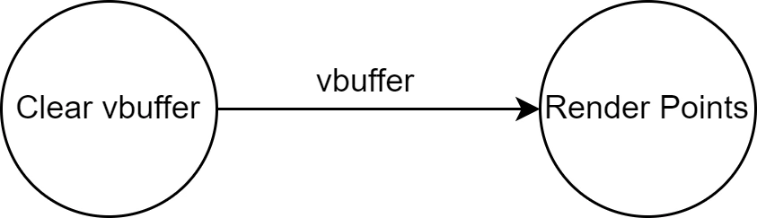
The visual representation of our render graph is quite basic and looks like this. What I have not added are all the resources that are not created by other nodes, as they are not relevant to the algorithms we apply to the graph later on.
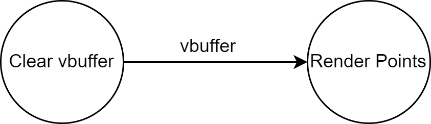
Simple example graph.
In order to illustrate the algorithms in the render graph a bit better, I am going to add some more nodes to our example graph. These would all be constructed with the same type of code as shown before. Mainly I am adding some passes that can run in parallel and a pass whose output is not used for the final image.
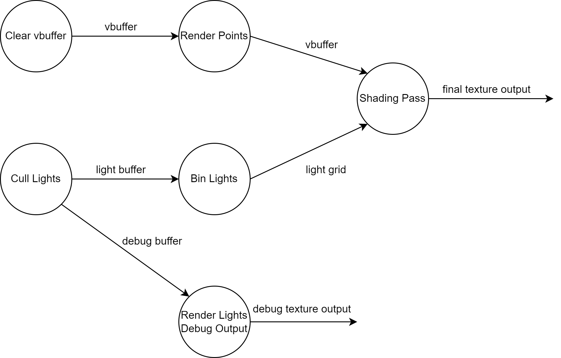
More advanced example graph to illustrate the algorithms
Dead Stripping
The process of removing all nodes that do not contribute to our final output is called dead stripping. It’s a technique that’s also common in compilers to remove code that does not do anything. The algorithm works by starting at the final output, and then walking through the graph and marking all the nodes that are visited as alive. In the end, we simply remove any nodes that we did not visit from the graph.
In our example graph, we start with the ‘final texture output’. That is created by ‘Shading Pass’, so we mark it as alive. Then we look at what read dependencies ‘Shading Pass’ has. It’s ‘vbuffer’, ‘light grid’. So we traverse to the ‘Render Points’ and ‘Bin Lights’ nodes, and mark them alive as well. And lastly, we visit each of the nodes that create the inputs for these nodes, ‘Clear vbuffer’ and ‘Cull Lights’, and mark them as alive as well. Since these nodes have no inputs created from other nodes we are done traversing. The only node we have not visited is the ‘Render Lights Debout Output’ node, so we can safely remove it from the graph. This makes our graph look like the following.
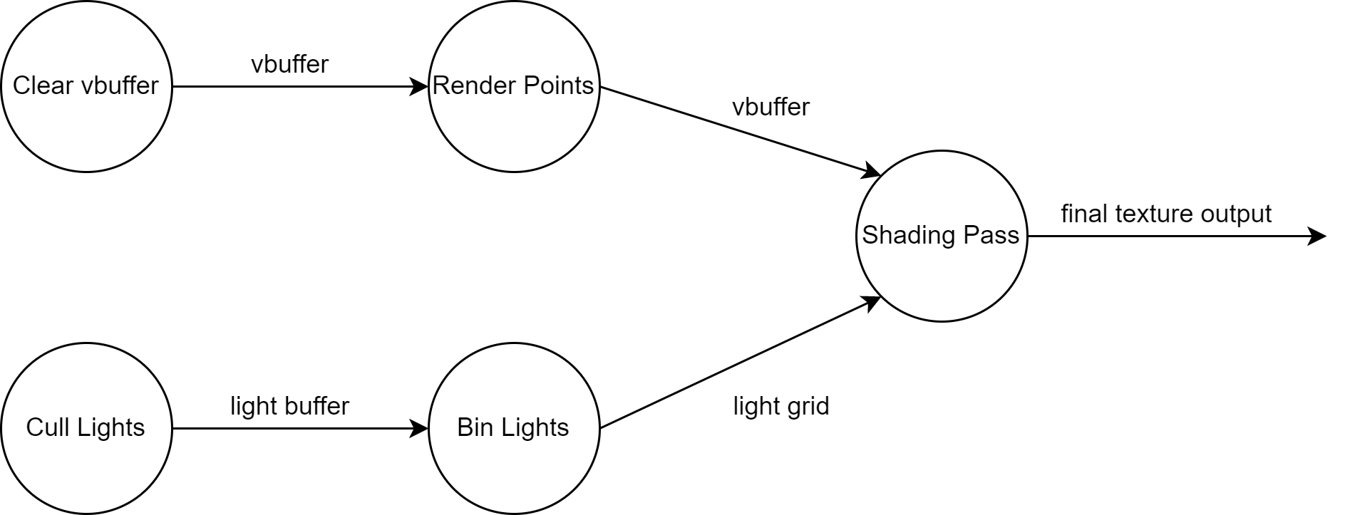
Example graph after dead stripping
Topology Sorting
In order to find out where memory barriers need to be placed, we can do a topology sort. This algorithm is also commonly found in compilers for determining in what order files need to be compiled. The output of our topology sort will be a list of lists. Each sub-list will contain nodes that can be recorded onto the command buffer without the need for a memory barrier in between. Only between the sub-lists is a memory barrier required. In our example graph the sorted list will look like the following:
[
    [ Clear vbuffer, Cull Lights ],
    [ Render Points, Bin Lights ],
    [ Shading Pass ],
]
Topology sort works by starting at all the nodes that have read dependencies. In our example, those are ‘Clear vbuffer’ and ‘Cull Lights’. We then remove these nodes from the graph, add these as a list to the list of lists, and repeat the process. We will find new nodes without dependencies since we have removed the nodes we just processed from the graph. If we don’t find any nodes without dependencies we are done processing. If there are still nodes left in the graph though, it means there are circular dependencies, which would indicate a bug in your render graph.
Executing the Render Graph
Now that the render graph is sorted, we can execute the nodes and record them on the command buffer. We simply loop through the list of lists we created with the topology sort and add a memory barrier between the sub-lists. One of the things I have not talked about is resource transitions. In our framework, we currently let the render-backend deal with those using minimal state tracking. However, the render graph does have all the information that you would need to do resource transitions.
Wrapping Up
In this blog post, I have given you an introduction to the concept of a render graph, the advantages that it can give us, and how some of the underlying algorithms work to make this possible.
I did not manage to talk about resource overlapping yet, since we have yet to implement that in our own framework. Right now we simply create all the resources and create a mapping from the resource handle index to the resource. Once we do have smarter resource allocation with overlapping you can expect a follow-up article with details on how that is implemented.
Some other things I would like to explore in the future are removing useless copies, scheduling work on an async compute queue, and recording on multiple command buffers in parallel.
Finally, there are some things I would like to mention, but could not quite fit in this post, so I have added them as bonuses.
Bonus I: Rasterization
We also want to be able to do rasterization with the render graph. For this we use a RasterPass node, which allows us to also bind render and depth stencil targets. In the current form, we only support a single draw call per pass, but we are looking into designing a nice API that allows doing many draw calls in an efficient manner.
Code sample — see the original on Medium, linked at the end of this post.
Bonus II: Custom Pass
Another nice feature we have in our render graph is that we can access the low-level API quite easily by creating a custom node. This is important for us if we for example need to create a quick prototype or want to try out a new Vulkan extension.
The custom node works by passing a closure which we call when we execute the compiled render graph.
Code sample — see the original on Medium, linked at the end of this post.
Further reading material
- https://www.gdcvault.com/play/1024612/FrameGraph-Extensible-Rendering-Architecture-in
- https://themaister.net/blog/2017/08/15/render-graphs-and-vulkan-a-deep-dive/
- https://ourmachinery.com/post/high-level-rendering-using-render-graphs/
- https://github.com/EmbarkStudios/kajiya/tree/main/crates/lib/kajiya-rg