Creating a Directed Acyclic Graph from a Mesh

In this post, we’d like to walk you through the steps of creating a Directed Acyclic Graph, or DAG, that we use at Traverse Research for our in-house rendering framework, Breda, to do mirco-polygon rendering. This is achieved by creating meshlets out of a larger mesh and iteratively joining and simplifying them. It can be used to stream, cull and render meshes at different levels of detail. While the general idea is similar to Unreal’s Nanite, their implementation is tailored to rasterization, while our focus will be primarily placed on raytracing. However, you will find that the steps as explained in this post are equally applicable to both.

This post assumes that the reader is somewhat familiar with mesh rendering on different levels of detail and rendering nomenclature, has a very rough idea about what Nanite tries to achieve, but otherwise requires no in-depth knowledge about Nanite or similar systems.

Introduction: Level of Detail, and the DAG

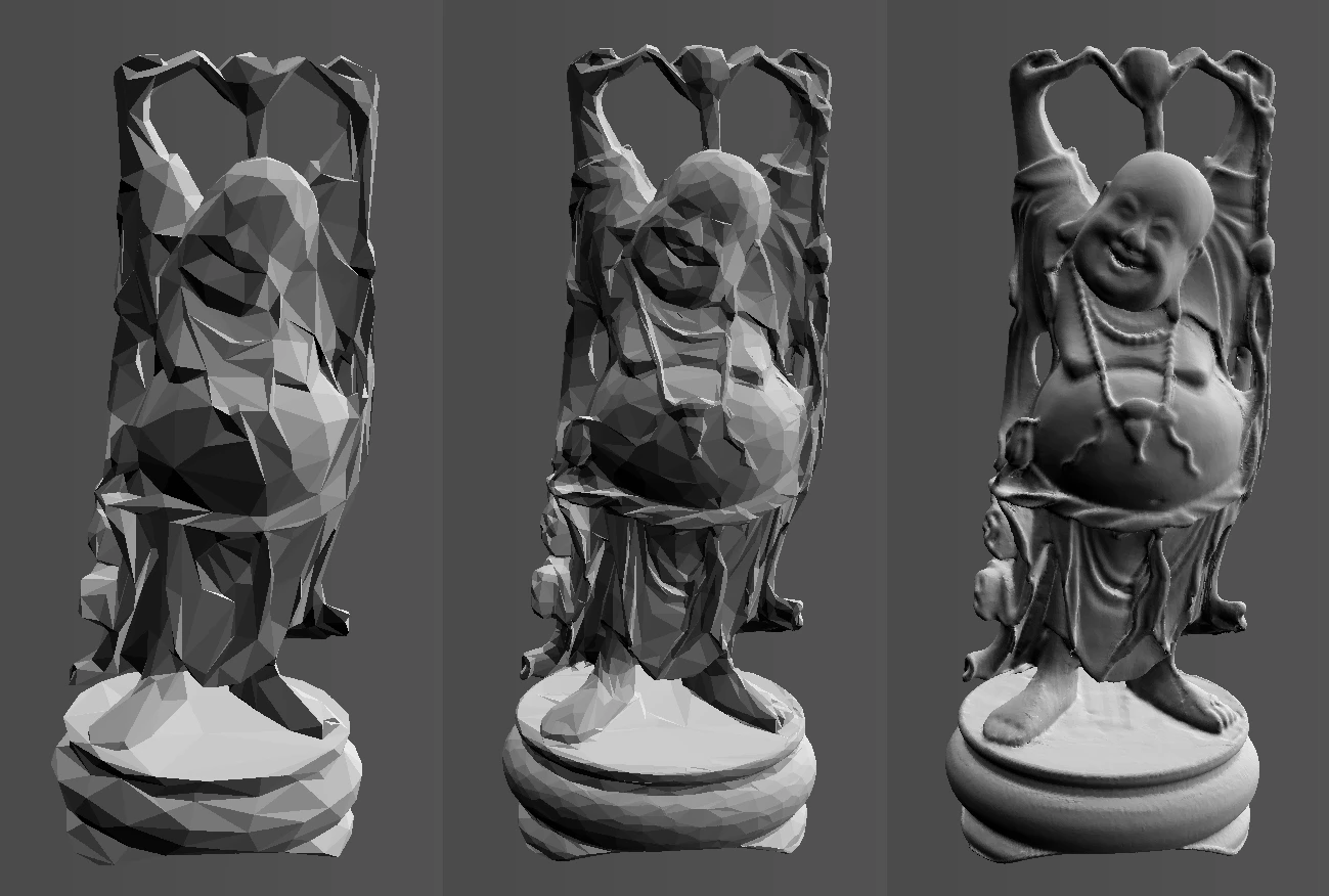
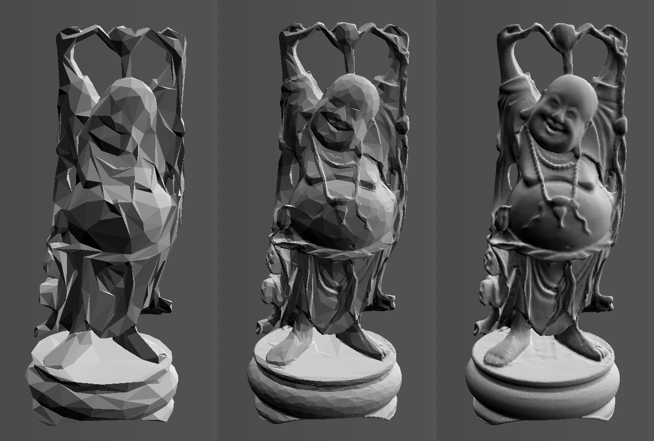
Stanford Buddha in three different levels of detail

There are several techniques to render meshes at several levels of detail, or LODs. Discussing them is beyond the scope of this post, but suffice to say is that most of them work on meshes as a whole. This isn’t particularly convenient for very large meshes such as landscapes and structures. You can split them up into smaller meshlets, but you’ll need to take extra care that any adjacent polygons sharing an edge between the meshlets will not cause any visible seams. This typically means that you somehow ensure that the polygons of either side use binary identical vertices, and that the edges between the verts are not more subdivided for one side than the other.

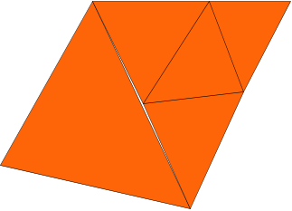
Adjacent polygons showing a seam as the right triangle is more subdivided than the left

One way to solve this problem is to never simplify the boundary of a meshlet. You could separate your mesh into a list of meshlets, and then recursively take two adjacent meshlets, combine them, and simplify them. You will end up with a tree structure, where each node in the tree is a simplified version of its two children combined. The collection of all leaf nodes represents the mesh at the highest level of detail, while the root node is the entire mesh at the lowest possible resolution.

But herein lies a problem. Remember how we never simplified the boundaries of meshlets. Of course, when pairing up adjacent meshlets, those edges that were considered a boundary at a higher resolution are now on the interior of the combined pair, so the edges do eventually end up simplified. However, if we consider the root node of the tree and its two children, the edges adjoining the two children have never been simplified. They are still at the resolution of the original mesh.

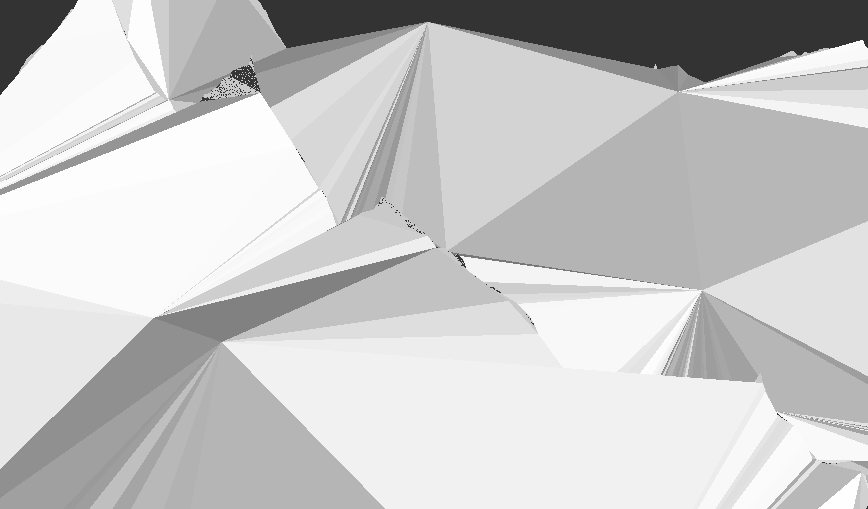
Heavily LODed terrain that shows a high-resolution split between two nodes

This is an inherent problem of tree structures. Because of their nature, you will always be able to draw a line separating the left side of the tree from the right.

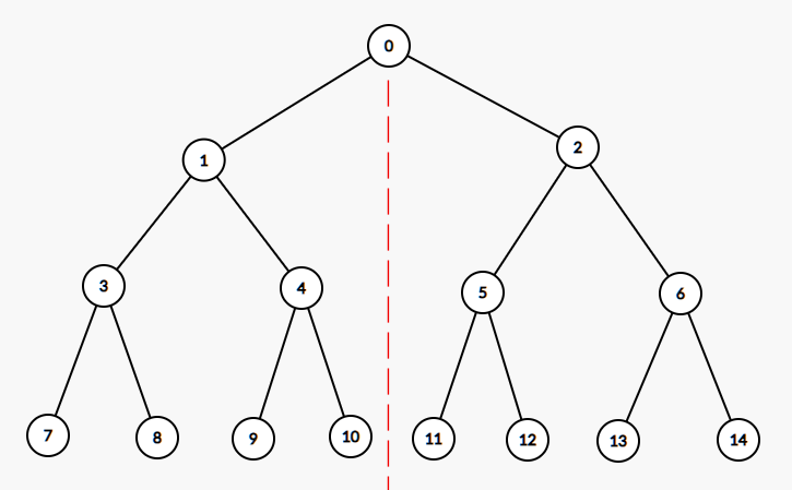
The red dashed line separates the left subtree from the right

What we need is some data structure where we can have connections between the nodes that straddle this line of separation. This is where the Directed Acyclic Graph, or DAG, comes in. It is a type of graph where the edges always point in a certain direction (hence “directed”), and when walking the edges from an arbitrary starting position you will never end up at the node where you started (hence “acyclic”). This would then look something like this:

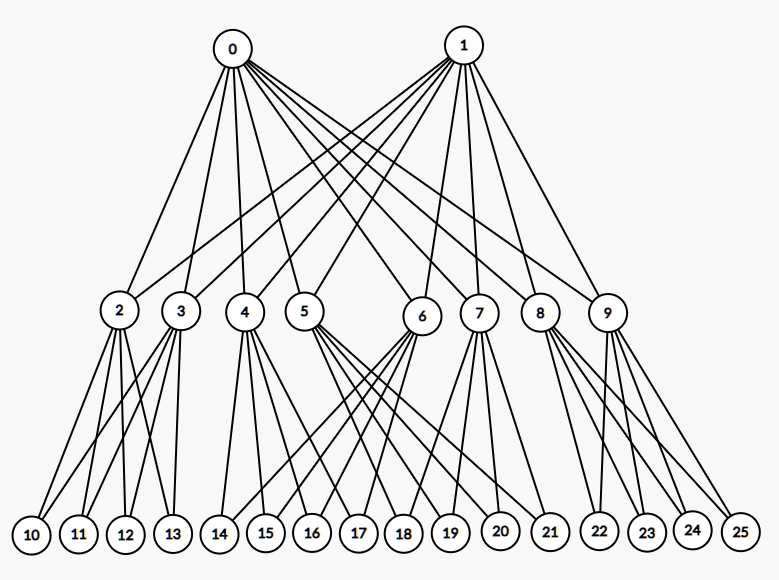
A directed acyclic graph

Strictly speaking, a DAG is a generalization of a tree: all trees are DAGs, but not all DAGs are trees. But a DAG allows for more connections between the nodes than is possible in a tree. Where a non-root node in the tree points to a single parent, a non-root node in the DAG can point to multiple “parent” nodes. This means diamond shapes are now possible. For example, in the picture above, notice how node 0 connects to nodes 5 and 7, which in turn both connect to node 18. Any border that 5 and 7 share, has been simplified before as there is no way to draw a line separating their child nodes.

But how to we achieve multiple parents? What does this mean in the context for our mesh? Well, remember how a connection of multiple child nodes to a parent means those nodes got merged into a parent. Having multiple parents for the same set of child nodes would therefore imply that they got merged into both parents, but the parents are somehow distinct. We achieve this by not only merging the nodes, but also splitting the result.

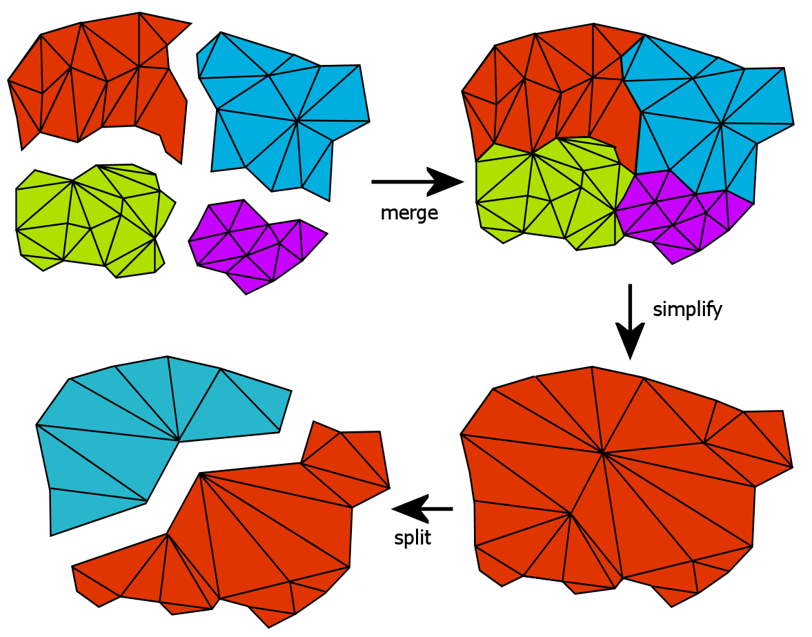
If we target a specific triangle count for each meshlet after the split, we need to merge more than two meshlets, the exact number depending on the simplification factor. For example, with a simplification factor of 0.5 (meaning a meshlet after simplification will have half the number of triangles), we need to merge 4 adjacent meshlets. To put it in other words, in order to target a fixed number of triangles per meshlet at each LOD, the simplification factor s is a function of the number of input i and output o meshlets: s = o / i

We feel that 4 inputs and 2 outputs, with a simplification factor of 0.5, is a decent balance. Your mileage may vary.

We should also consider that some nodes might never merge. This might be because of their spatial separation or other metrics you might use to consider nodes for merging. The DAG should be able to accommodate for this situation, and that means it should support multiple root nodes. Similarly, the number of meshlets will unlikely be always divisible by the amount of meshlets you want to merge, so the number of children for a non-leaf node in the DAG should not be a constant.

Creating the DAG

Now that we have a general idea of what our DAG is going to look like, we need to define some parameters. We’ve already discussed that we like to merge 4 meshlets and then split them into 2. Furthermore, we need to decide on a target triangle count per meshlet. For our particular use case at Traverse Research, we have chosen 1024. This value is not set in stone and still very subject to change. Since our framework heavily relies on raytracing, we need to generate bottom level acceleration structures (BLASes) to be able to ray-trace the mesh, so we need to find a balance between triangle count, memory overhead and runtime performance. A low triangle count results in a finer LOD granularity, but more BLAS memory overhead. It also results in a larger DAG, which might affect performance of the determination of the active cut. However, for other purposes, fewer or more triangles might be a better fit. Again, YMMV.

The algorithm to create a DAG out of a high-resolution mesh consists of the following steps:

// first, transform the mesh in a list of meshlets
let meshlets = generate_meshlets(mesh)

// and put them as leaf nodes in the dag
dag.add_leafs(meshlets)

// track all the borders between the meshlets
find_borders(meshlets)

// iteratively merge-simplify-split
while we can group meshlets:
  for group in partition(meshlets):
    // merge the meshlets in the group
    let meshlet = merge(group)

    // remove parts of border that is now on the inside of the merged meshlet
    update_border(meshlet)

    // simplify the merged meshlet
    simplify(meshlet)

    // split the simplified meshlet
    let parts = split(meshlet)

    // split the borders
    split_borders(parts)

    // write the result to the dag
    dag.add_parents(group, parts)

Third party tools

For our implementation, we have opted to use two open-source libraries.

The first is Meshoptimizer, which is a C library (Rust bindings available) to simplify the mesh, generate meshlets, and other useful mesh processing tools. Beware that its meshlet generation is specifically tailored to store the meshlets using very compact data format, and it therefore only supports at most 126 tris and 64 verts, which unfortunately is too low for our own goals.

For our simplification needs, we need to be able to specify which edges to lock to prevent the meshlet border from being simplified. A PR has been submitted to add this to the API, but unfortunately has not yet been merged at time of writing (Rust bindings exposing this feature available here)

We also use METIS, a C library (Rust bindings available) to partition a graph. We use this library to partition the list of meshlets into groups of N meshlets. In our experience, using METIS hasn’t always seemed very intuitive. In the last chapter of this post, we will go more in-depth on the relevant API functions and how to use them.

Generating the initial list of meshlets

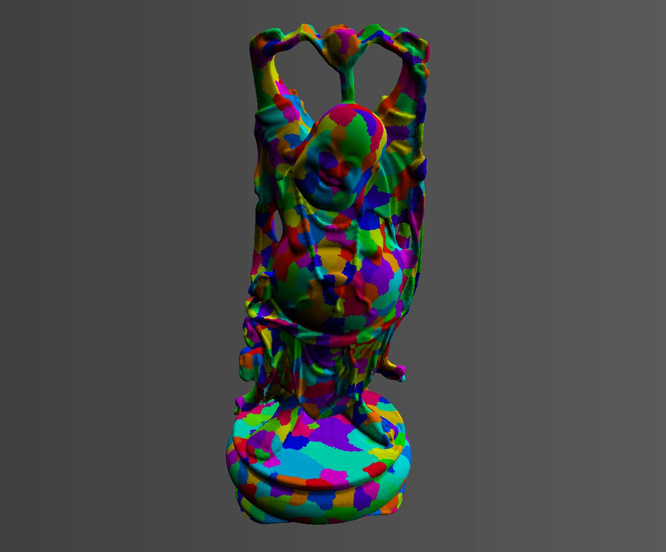
Generated meshlets for the Stanford Buddha

Given that the meshlet generator of the Meshoptimizer is not suitable for our triangle count, we use METIS here as well to partition the initial mesh into groups of 1024 triangles. One downside is that METIS only works on the topology of the graph; it has no knowledge about special coordinates of the vertices. This is usually fine for one large continuous mesh of roughly equally sized triangles, but if your input has an irregular shape, you might want to use a different algorithm. This is especially true if you want to group triangles in meshlets based on other properties, such as face normals.

Special care should be taken with parts of the mesh that are disjoint, especially when using METIS. You can merge disjoint parts into a single meshlet, but as METIS has no knowledge about spatial separation, our suggestion is to keep those separate and only use METIS to work on continuous meshes.

As we want to partition the graph of meshlets using METIS, we need to keep track of meshlet connectivity. We also need to track the borders shared between the meshlets, as this is both important for generating an optimal partition and for locking the border during simplification.

Tracking meshlet borders

Tracking borders might not be a straightforward problem, as we need to distinguish between the original mesh border that is allowed to be simplified, and the borders that we create by partitioning the mesh into meshlets.

For our algorithm, we define an edge as the connection between two vertices. As we’re working with vertex indices, it’s convenient to encode an edge simply as a tuple of two vertex indices: (i0, i1), where i0 < i1. The latter condition ensures that we can always uniquely identify the same edge, regardless of the order of vertex indices in the triangle. This way we can use it as a key in some kind of associated data structure such as a hash map.

Furthermore, we define a border as a list of edges that is shared between a pair of meshlets. A meshlet can have multiple borders (as it connects to multiple adjacent meshlets), but two meshlets only share a single border.

Initial border computation

To generate the initial borders for all meshlets:

// create a map of edges that maps an edge to a list of meshlets
define edge_map: map of edge -> list of meshlet
for meshlet in meshlets:
  for edge in edges(meshlet):
    edge_map[edge].add(meshlet)

// create a map of borders that maps a meshlet pair to a list of edges
define border_map: map of (meshlet, meshlet) -> list of edge
for (edge, meshlets) in edge_map:
  for meshlet_pair in all pairs in meshlets:
    border_map[meshlet_pair].add(edge)

// now that border_map contains a list of edges per pair of meshlets,
// we can add it to the meshlets
for (meshlet_pair, edges) in border_map:
  let b = new Border(edges, meshlet_pair)
  meshlet_pair[0].add_border(b)
  meshlet_pair[1].add_border(b)

With this code, we have generated an initial list of borders for each meshlet. As you might have spotted, both meshlets refer to the same border object. The reason for this becomes apparent as we split the meshlets after simplification. We also use these border objects as connectivity information; the meshlet pair of a border are connected to each other in the graph. So, in a sense, these borders themselves form the edges of the meshlet connectivity graph.

Updating the borders during merge-simplify-split

In the next phase of our algorithm, we iteratively find meshlet groups by partitioning the meshlet graph, and then for each group we merge the meshlets into one bigger meshlet, the merged meshlet, simplify the resulting meshlet into the simplified meshlet, and then split that meshlet into two parts, the split meshlets.

During merging, the inner border disappears. For the merged meshlet, we can collect all borders from the individual meshlets in the group, and remove those borders where both of the meshlet pairs are within the group.

define merged_borders: list of Border
for meshlet in group:
  for border in meshlet.borders:
    let (a, b) = border.meshlet_pair
    if not group.contains(a) or not group.contains(b):
      merged_borders.add(border)

After simplification, the outer border of the simplified meshlet remains untouched, as we locked it for simplification. However, as we split the simplified meshlet, we are very likely split an existing border! We need functionality to split a border, while keeping intact the connectivity information of the new split meshlets with its original adjacent meshlets. Also, we need to generate a whole new border for the split between the split meshlets.

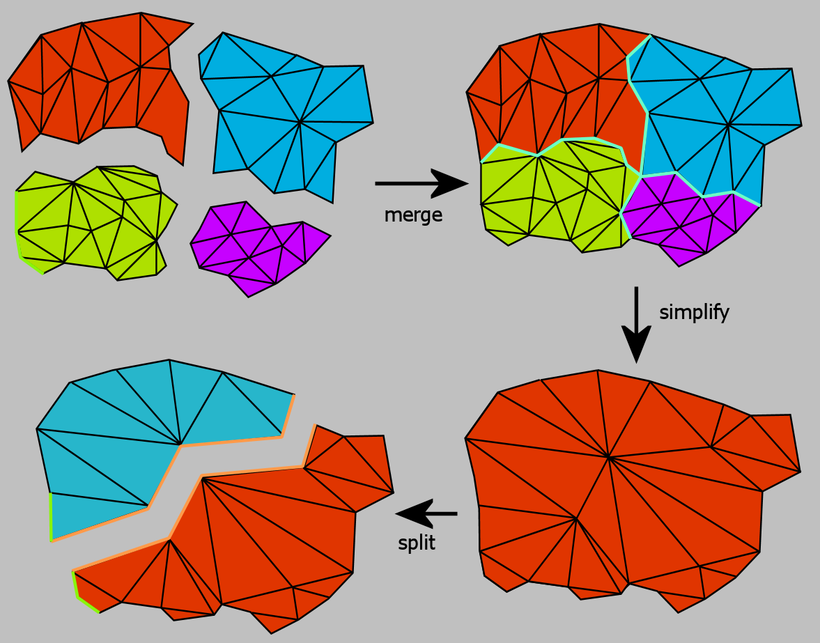
Another diagram showing the merge-simply-split process, this time highlighting some of the border cases. In the merged meshlet in the upper right, we see an inner border that can be removed highlighted in teal. The final split meshlets in the lower left show both a new border in orange and an original border (that was originally part of the green mesh) that is being split in green.

The general idea to solving this problem is to generate two sets of edges, A and B, one for each split meshlet. We can then walk over the borders of the merged meshlet, calculating the intersection of the border edges with either edge set. If either 0 or all of the border edges are in set A, the border remains unsplit. If some are in set A and some in set B, we need to split the border and update the references. The new border between the split meshlets is simply the intersection of A and B.

// first, let’s define some supporting functions

// this function checks whether one of the pair of meshlets is
// contained in the group, and if so, it updates its reference to
// the new meshlet
fn update_meshlet(border, group, new_meshlet):
  if group.contains(border.meshlet_pair[0]):
    border.meshlet_pair[0] = new_meshlet
  else:
    border.meshlet_pair[1] = new_meshlet

// this function splits the border into two, based on a set of edges belonging to
// split_meshlets[0].
// it also requires a group of meshlets that contains one of the elements
// of the original border’s meshlet pairs, and a new pair of split meshlets
fn split_border(border, edges, group, split_meshlets):
  // remove all edges not contained in the ‘edges’ set, and move them to a separate list
  let other_edges = border.edges.retain(edges)
  let other_border = new Border(other_edges, border.meshlet_pair)
  update_meshlet(border, group, split_meshlets[0])
  split_meshlets[0].add_border(border)
  update_meshlet(other_border, group, split_meshlets[1])
  split_meshlets[1].add_border(other_border)

// update all borders
let edges_a = set of edges in split_meshlets[0]
let edges_b = set of edges in split_meshlets[1]

let b = new Border(intersection(edges_a, edges_b), split_meshlets)
split_meshlet[0].add_border(b);
split_meshlet[1].add_border(b);

for border in merged_borders:
  let i = intersection(edges_a, border.edges)
  if count(i) = count(border.edges):
    // border is completely in A
    // this function checks which of the meshlet pair is in the group, and then
    // updates that reference accordingly
    update_meshlet(border, group, split_meshlets[0])
    split_meshes[0].add_border(border);
  else if count(i) = 0:
    // border is completely in B
    update_meshlet(border, group, split_meshlets[1])
    split_meshes[1].add_border(border);
  else:
    // this function splits the border based on an edge set, and
    // updates internal references. After this call, the adjacent meshlet not
    // part of the group will contain both pieces of split border
    split_border(border, a, group, split_meshlets)

After all groups of meshlets have been merged, simplified and split, the borders are all updated and will point to the new split meshlets.

And there we have it. After we have determined there are no more meshlets to group, we have filled the entire DAG, and the root nodes are now heavily simplifed representations of the mesh.

Determining the cut of the DAG

Now that we generated the DAG, we need to select which nodes we’re interested in rendering. These node are what’s called the cut of the DAG. We need some kind of metric to determine which DAG nodes are below the quality threshold (0) and which are above (1). But remember, this is not a tree. Because of the nature of the DAG, there are many paths from a root to a certain node, so we cannot simply recursively walk the DAG and evaluate nodes as we encounter them. For an efficient (and parallelizable) implementation, we should be able to walk over all connections between parent and child in arbitrary order, and evaluate whether that child should render, without considering any other information.

To generate a correct cut, our evaluation function should adhere to some conditions:

• Given an arbitrary path from a root to a leaf node, the evaluation function should only flip from 0 to 1 once. All ancestors above the flip should report 0, all descendants below the flip should report 1. In other words, the evaluation of nodes should always be monotonically increasing.
• All parents of a single node should always evaluate the same. Remember that these parents represent the split parts of a merged & simplified piece of mesh. If the evaluation function determines that parent A should render but parent B should not, and all the children of parent B render instead, then there will be visible overlap between parent A itself and parent B’s children.

Given these specifications, the cut is then simply defined as each child node that evaluates to 1 where its parents evaluates to 0.

Finding a good and correct metric for the evaluation function is hard. For rasterization, you could determine the projected on-screen error given an error metric calculated during simplification. With raytracing, this is a harder problem because you can’t easily evaluate an object’s projected screen size. So for us this is still an open question.

Conclusion

This concludes this blog post. We went over the DAG creation algorithm, together with some more in-depth techniques to track mesh borders, and how you would go about to selecting a cut.

Here’s a little demo of what we did at Traverse:

Code sample — see the original on Medium, linked at the end of this post.

This post has been written by Sylvester Hesp at Traverse Research. If you have any questions or remarks, feel free to reach out through our website.